.ipynb .pdf

repository open issue

Binder

Contents

13. Models with Memory

# Install packages that are not installed in colab
try:
  import google.colab
  %pip install -q watermark
  %pip install git+https://github.com/ksachdeva/rethinking-tensorflow-probability.git  
except:
  pass

%load_ext watermark

# Core
import numpy as np
import arviz as az
import pandas as pd
import xarray as xr
import tensorflow as tf
import tensorflow_probability as tfp

# visualization
import matplotlib.pyplot as plt

from rethinking.data import RethinkingDataset
from rethinking.data import dataframe_to_tensors
from rethinking.mcmc import sample_posterior


# aliases
tfd = tfp.distributions
tfb = tfp.bijectors
Root = tfd.JointDistributionCoroutine.Root

2022-01-19 19:13:29.224239: W tensorflow/stream_executor/platform/default/dso_loader.cc:64] Could not load dynamic library 'libcudart.so.11.0'; dlerror: libcudart.so.11.0: cannot open shared object file: No such file or directory
2022-01-19 19:13:29.224278: I tensorflow/stream_executor/cuda/cudart_stub.cc:29] Ignore above cudart dlerror if you do not have a GPU set up on your machine.

%watermark -p numpy,tensorflow,tensorflow_probability,arviz,scipy,pandas,rethinking

numpy                 : 1.21.5
tensorflow            : 2.7.0
tensorflow_probability: 0.15.0
arviz                 : 0.11.4
scipy                 : 1.7.3
pandas                : 1.3.5
rethinking            : 0.1.0

# config of various plotting libraries
%config InlineBackend.figure_format = 'retina'

13.1 Example: Multilevel tadpoles

Code 13.1

Reedfrogs dataset is about the tadpole mortality. The objective will be determine the surv out of an initial count, density.

Author explains that within each tank there are things that go unmeasured and these unmeasured factors create variation in survival across tanks.

These tanks are an example of cluster variable

He argues that both of the approaches - * treat the tanks independetly i.e. each of them have their unique intecepts * treat them togather

have issues.

for e.g.

- unique intecepts will imply that we are not using information from other tanks.
- all togather will have the problem ignoring varations in baseline survival 

A multilevel model, in which we simultaneously estimate both an intercept for each tank and the variation among tanks, is what we want !

This type of a model is called Varying intercepts model.

d = RethinkingDataset.ReedFrogs.get_dataset()
d.head()

	density	pred	size	surv	propsurv
0	10	no	big	9	0.9
1	10	no	big	10	1.0
2	10	no	big	7	0.7
3	10	no	big	10	1.0
4	10	no	small	9	0.9

Code 13.2

Our simple model. This will give us 48 different intercepts. This means that it does not use the information available between each tank

d["tank"] = np.arange(d.shape[0])
alpha_sample_shape = d["tank"].shape[0]

# dat = dict(
#     S=tf.cast(d.surv.values, dtype=tf.float32),
#     N=tf.cast(d.density.values, dtype=tf.float32),
#     tank=d.tank.values)

tdf = dataframe_to_tensors(
    "ReedFrogs", d, {"tank": tf.int32, "surv": tf.float32, "density": tf.float32}
)


def model_13_1(tid, density):
    def _generator():
        alpha = yield Root(
            tfd.Sample(tfd.Normal(loc=0.0, scale=1.5), sample_shape=alpha_sample_shape)
        )
        p = tf.sigmoid(tf.squeeze(tf.gather(alpha, tid, axis=-1)))

        S = yield tfd.Independent(
            tfd.Binomial(total_count=density, probs=p), reinterpreted_batch_ndims=1
        )

    return tfd.JointDistributionCoroutine(_generator, validate_args=False)


jdc_13_1 = model_13_1(tdf.tank, tdf.density)

2022-01-19 19:13:32.168212: W tensorflow/stream_executor/platform/default/dso_loader.cc:64] Could not load dynamic library 'libcuda.so.1'; dlerror: libcuda.so.1: cannot open shared object file: No such file or directory
2022-01-19 19:13:32.168253: W tensorflow/stream_executor/cuda/cuda_driver.cc:269] failed call to cuInit: UNKNOWN ERROR (303)
2022-01-19 19:13:32.168278: I tensorflow/stream_executor/cuda/cuda_diagnostics.cc:156] kernel driver does not appear to be running on this host (fv-az272-145): /proc/driver/nvidia/version does not exist
2022-01-19 19:13:32.168607: I tensorflow/core/platform/cpu_feature_guard.cc:151] This TensorFlow binary is optimized with oneAPI Deep Neural Network Library (oneDNN) to use the following CPU instructions in performance-critical operations:  AVX2 FMA
To enable them in other operations, rebuild TensorFlow with the appropriate compiler flags.

NUM_CHAINS_FOR_13_1 = 2

init_state = [tf.zeros([NUM_CHAINS_FOR_13_1, alpha_sample_shape])]

bijectors = [tfb.Identity()]

posterior_13_1, trace_13_1 = sample_posterior(
    jdc_13_1,
    observed_data=(tdf.surv,),
    params=["alpha"],
    num_chains=NUM_CHAINS_FOR_13_1,
    init_state=init_state,
    bijectors=bijectors,
)

az.summary(trace_13_1, round_to=2, kind="all", hdi_prob=0.89)

WARNING:tensorflow:@custom_gradient grad_fn has 'variables' in signature, but no ResourceVariables were used on the forward pass.

	mean	sd	hdi_5.5%	hdi_94.5%	mcse_mean	mcse_sd	ess_bulk	ess_tail	r_hat
alpha[0]	1.73	0.76	0.58	2.95	0.03	0.02	869.65	528.73	1.01
alpha[1]	2.42	0.88	0.98	3.66	0.04	0.03	487.27	316.79	1.00
alpha[2]	0.78	0.65	-0.17	1.85	0.02	0.02	1427.46	469.72	1.01
alpha[3]	2.37	0.89	0.92	3.60	0.03	0.03	673.36	480.56	1.01
alpha[4]	1.72	0.75	0.49	2.81	0.03	0.02	681.85	548.39	1.00
alpha[5]	1.70	0.74	0.60	2.89	0.03	0.02	687.96	446.64	1.00
alpha[6]	2.44	0.92	0.96	3.75	0.04	0.03	517.86	519.91	1.00
alpha[7]	1.70	0.78	0.64	3.07	0.03	0.02	641.05	321.61	1.00
alpha[8]	-0.38	0.63	-1.32	0.73	0.02	0.03	1038.50	351.14	1.02
alpha[9]	1.73	0.78	0.37	2.80	0.03	0.02	751.08	431.66	1.00
alpha[10]	0.76	0.62	-0.10	1.80	0.02	0.02	911.38	348.36	1.00
alpha[11]	0.37	0.58	-0.52	1.22	0.02	0.02	1324.36	436.95	1.01
alpha[12]	0.76	0.61	-0.34	1.59	0.02	0.02	868.90	397.02	1.01
alpha[13]	0.02	0.55	-0.86	0.83	0.01	0.03	1397.55	352.09	1.00
alpha[14]	1.72	0.75	0.60	2.92	0.03	0.02	747.66	439.10	1.02
alpha[15]	1.75	0.72	0.62	2.77	0.03	0.02	622.83	516.00	1.00
alpha[16]	2.55	0.67	1.50	3.54	0.02	0.02	836.00	424.08	1.00
alpha[17]	2.13	0.57	1.20	2.92	0.02	0.01	1019.37	248.43	1.01
alpha[18]	1.80	0.53	1.05	2.68	0.02	0.01	1172.29	271.93	1.02
alpha[19]	3.12	0.79	1.91	4.35	0.03	0.02	748.37	554.95	1.00
alpha[20]	2.13	0.63	1.16	3.12	0.02	0.01	1127.72	367.52	1.01
alpha[21]	2.18	0.60	1.19	3.04	0.02	0.02	1195.55	333.55	1.01
alpha[22]	2.14	0.56	1.24	2.94	0.02	0.01	1275.19	379.52	1.01
alpha[23]	1.57	0.55	0.64	2.40	0.02	0.02	1110.26	103.62	1.01
alpha[24]	-1.11	0.48	-1.87	-0.29	0.01	0.02	1489.06	61.64	1.06
alpha[25]	0.08	0.38	-0.49	0.71	0.01	0.02	1396.74	392.23	1.00
alpha[26]	-1.53	0.49	-2.32	-0.81	0.01	0.01	1782.69	154.20	1.02
alpha[27]	-0.57	0.38	-1.07	0.09	0.01	0.01	1093.14	215.15	1.00
alpha[28]	0.08	0.39	-0.58	0.66	0.01	0.02	1446.12	302.73	1.00
alpha[29]	1.32	0.40	0.79	1.86	0.01	0.02	1756.26	90.07	1.01
alpha[30]	-0.71	0.47	-1.39	0.10	0.01	0.02	1584.68	213.10	1.01
alpha[31]	-0.40	0.42	-1.09	0.21	0.01	0.02	1435.74	262.31	1.01
alpha[32]	2.86	0.64	1.75	3.78	0.02	0.02	1243.66	421.61	1.00
alpha[33]	2.47	0.63	1.54	3.53	0.02	0.02	1392.94	204.56	1.04
alpha[34]	2.47	0.59	1.64	3.56	0.02	0.01	1638.33	176.87	1.02
alpha[35]	1.92	0.42	1.18	2.52	0.01	0.01	1453.83	186.40	1.01
alpha[36]	1.89	0.49	1.13	2.66	0.01	0.01	1464.74	43.66	1.12
alpha[37]	3.37	0.82	2.06	4.67	0.04	0.03	587.52	499.66	1.00
alpha[38]	2.45	0.52	1.56	3.16	0.02	0.01	1318.07	386.09	1.00
alpha[39]	2.17	0.59	1.31	3.08	0.02	0.01	1918.12	146.95	1.02
alpha[40]	-1.90	0.48	-2.64	-1.14	0.01	0.01	1337.42	108.70	1.04
alpha[41]	-0.63	0.34	-1.20	-0.15	0.01	0.01	842.19	587.31	1.00
alpha[42]	-0.49	0.34	-0.93	0.09	0.01	0.01	851.03	714.36	1.00
alpha[43]	-0.38	0.33	-0.88	0.19	0.01	0.01	742.51	733.94	1.01
alpha[44]	0.54	0.35	0.01	1.14	0.01	0.01	901.53	563.61	1.00
alpha[45]	-0.62	0.35	-1.12	0.01	0.01	0.01	762.64	415.80	1.01
alpha[46]	1.92	0.50	0.99	2.60	0.02	0.02	1216.79	60.88	1.04
alpha[47]	-0.05	0.34	-0.56	0.51	0.01	0.01	843.78	696.34	1.00

Code 13.3

We now build a multilevel model, which adaptively pools information across tanks.

In order to do so, we must make the prior for the parameter alpha a function of some new parameters.

Prior itself has priors !

def model_13_2(tid, density):
    def _generator():
        a_bar = yield Root(tfd.Sample(tfd.Normal(loc=0.0, scale=1.5), sample_shape=1))
        sigma = yield Root(tfd.Sample(tfd.Exponential(rate=1.0), sample_shape=1))
        alpha = yield tfd.Sample(
            tfd.Normal(loc=a_bar, scale=sigma), sample_shape=alpha_sample_shape
        )
        p = tf.sigmoid(tf.squeeze(tf.gather(alpha, tid, axis=-1)))

        S = yield tfd.Independent(
            tfd.Binomial(total_count=density, probs=p), reinterpreted_batch_ndims=1
        )

    return tfd.JointDistributionCoroutine(_generator, validate_args=False)


jdc_13_2 = model_13_2(tdf.tank, tdf.density)

NUM_CHAINS_FOR_13_2 = 2

init_state = [
    tf.zeros([NUM_CHAINS_FOR_13_2]),
    tf.ones([NUM_CHAINS_FOR_13_2]),
    tf.zeros([NUM_CHAINS_FOR_13_2, alpha_sample_shape]),
]

bijectors = [tfb.Identity(), tfb.Exp(), tfb.Identity()]

posterior_13_2, trace_13_2 = sample_posterior(
    jdc_13_2,
    observed_data=(tdf.surv,),
    params=["a_bar", "sigma", "alpha"],
    num_chains=NUM_CHAINS_FOR_13_2,
    init_state=init_state,
    bijectors=bijectors,
)

az.summary(trace_13_2, round_to=2, kind="all", hdi_prob=0.89)

	mean	sd	hdi_5.5%	hdi_94.5%	mcse_mean	mcse_sd	ess_bulk	ess_tail	r_hat
a_bar	1.34	0.25	0.96	1.75	0.01	0.01	386.35	270.34	1.01
sigma	1.62	0.21	1.28	1.91	0.02	0.02	83.87	79.97	1.03
alpha[0]	2.13	0.91	0.75	3.62	0.10	0.07	91.84	166.86	1.02
alpha[1]	3.20	1.06	1.28	4.59	0.22	0.16	24.69	66.83	1.10
alpha[2]	0.99	0.71	-0.09	2.08	0.06	0.04	150.07	214.84	1.01
alpha[3]	3.01	1.01	1.43	4.75	0.11	0.08	80.13	153.60	1.01
alpha[4]	2.19	0.92	0.72	3.39	0.10	0.07	102.60	134.35	1.03
alpha[5]	2.28	0.92	0.95	3.86	0.09	0.06	105.92	229.54	1.00
alpha[6]	3.06	0.98	1.45	4.43	0.13	0.09	60.49	120.60	1.02
alpha[7]	2.27	0.77	1.10	3.45	0.07	0.05	127.68	176.14	1.03
alpha[8]	-0.17	0.61	-1.09	0.89	0.05	0.03	178.89	339.49	1.01
alpha[9]	2.12	0.81	0.75	3.31	0.09	0.06	83.05	177.11	1.02
alpha[10]	1.00	0.67	-0.01	2.09	0.05	0.04	170.56	243.76	1.01
alpha[11]	0.60	0.65	-0.37	1.59	0.05	0.04	151.85	199.69	1.00
alpha[12]	0.99	0.69	-0.10	1.99	0.08	0.06	85.77	91.97	1.02
alpha[13]	0.20	0.59	-0.59	1.24	0.04	0.03	261.52	362.34	1.00
alpha[14]	2.12	0.78	0.90	3.32	0.07	0.05	139.83	220.11	1.03
alpha[15]	2.21	0.93	0.93	3.62	0.14	0.11	56.41	41.22	1.04
alpha[16]	2.63	0.72	1.53	3.68	0.07	0.05	114.22	131.00	1.01
alpha[17]	2.41	0.63	1.55	3.53	0.05	0.04	147.74	272.04	1.01
alpha[18]	2.02	0.61	1.07	2.91	0.05	0.03	187.76	214.88	1.01
alpha[19]	3.61	1.00	2.21	5.12	0.13	0.10	72.55	74.34	1.06
alpha[20]	2.39	0.71	1.28	3.49	0.06	0.04	161.41	266.01	1.01
alpha[21]	2.42	0.64	1.38	3.30	0.05	0.04	147.40	187.06	1.01
alpha[22]	2.43	0.67	1.34	3.35	0.05	0.03	200.50	272.25	1.01
alpha[23]	1.71	0.52	0.89	2.51	0.03	0.02	281.51	348.62	1.01
alpha[24]	-1.03	0.45	-1.70	-0.28	0.02	0.02	358.82	397.34	1.00
alpha[25]	0.15	0.39	-0.43	0.80	0.02	0.01	519.57	682.40	1.00
alpha[26]	-1.44	0.50	-2.31	-0.72	0.03	0.02	268.08	403.02	1.00
alpha[27]	-0.48	0.40	-1.15	0.10	0.02	0.01	479.73	495.67	1.00
alpha[28]	0.18	0.41	-0.57	0.73	0.02	0.01	529.31	644.48	1.00
alpha[29]	1.44	0.49	0.58	2.16	0.03	0.02	338.23	401.31	1.01
alpha[30]	-0.65	0.41	-1.30	-0.04	0.02	0.01	440.17	549.16	1.00
alpha[31]	-0.34	0.43	-0.99	0.33	0.02	0.02	322.09	372.26	1.00
alpha[32]	3.26	0.79	2.02	4.46	0.07	0.05	145.70	279.94	1.01
alpha[33]	2.74	0.68	1.67	3.74	0.05	0.04	177.04	398.17	1.02
alpha[34]	2.67	0.60	1.77	3.65	0.05	0.03	171.55	251.28	1.01
alpha[35]	2.06	0.51	1.28	2.82	0.03	0.02	282.35	377.61	1.00
alpha[36]	2.02	0.50	1.30	2.80	0.03	0.02	310.15	279.33	1.00
alpha[37]	3.91	0.92	2.43	5.26	0.11	0.08	66.18	151.03	1.01
alpha[38]	2.74	0.65	1.76	3.77	0.07	0.05	111.59	178.48	1.00
alpha[39]	2.36	0.57	1.46	3.20	0.04	0.03	214.46	238.12	1.01
alpha[40]	-1.83	0.50	-2.52	-0.98	0.03	0.02	244.82	188.28	1.01
alpha[41]	-0.55	0.35	-1.14	-0.05	0.01	0.01	642.74	585.39	1.00
alpha[42]	-0.46	0.35	-1.01	0.12	0.01	0.01	689.95	587.12	1.00
alpha[43]	-0.34	0.34	-0.83	0.22	0.01	0.01	821.89	614.02	1.00
alpha[44]	0.59	0.37	0.07	1.25	0.02	0.01	566.28	404.61	1.00
alpha[45]	-0.57	0.36	-1.11	0.02	0.01	0.01	634.35	459.83	1.01
alpha[46]	2.06	0.48	1.37	2.83	0.04	0.03	182.37	334.85	1.01
alpha[47]	0.02	0.32	-0.48	0.52	0.01	0.01	823.96	556.82	1.00

Code 13.4

# we must compute the likelhood before using arviz to do comparison
def compute_and_store_log_likelihood_for_model_13_1():

    sample_alpha = posterior_13_1["alpha"]

    ds, _ = jdc_13_1.sample_distributions(value=[sample_alpha, None])

    log_likelihood_13_1 = ds[-1].distribution.log_prob(tdf.surv).numpy()

    # we need to insert this in the sampler_stats
    sample_stats_13_1 = trace_13_1.sample_stats

    coords = [
        sample_stats_13_1.coords["chain"],
        sample_stats_13_1.coords["draw"],
        np.arange(48),
    ]

    sample_stats_13_1["log_likelihood"] = xr.DataArray(
        log_likelihood_13_1,
        coords=coords,
        dims=["chain", "draw", "log_likelihood_dim_0"],
    )


compute_and_store_log_likelihood_for_model_13_1()

def compute_and_store_log_likelihood_for_model_13_2():

    sample_abar = posterior_13_2["a_bar"]
    sample_sigma = posterior_13_2["sigma"]
    sample_alpha = posterior_13_2["alpha"]

    ds, _ = jdc_13_2.sample_distributions(
        value=[sample_abar, sample_sigma, sample_alpha, None]
    )

    log_likelihood_13_2 = ds[-1].distribution.log_prob(tdf.surv).numpy()

    # we need to insert this in the sampler_stats
    sample_stats_13_2 = trace_13_2.sample_stats

    coords = [
        sample_stats_13_2.coords["chain"],
        sample_stats_13_2.coords["draw"],
        np.arange(48),
    ]

    sample_stats_13_2["log_likelihood"] = xr.DataArray(
        log_likelihood_13_2,
        coords=coords,
        dims=["chain", "draw", "log_likelihood_dim_0"],
    )


compute_and_store_log_likelihood_for_model_13_2()

az.compare({"m13.1": trace_13_1, "m13.2": trace_13_2})

/opt/hostedtoolcache/Python/3.7.12/x64/lib/python3.7/site-packages/arviz/stats/stats.py:695: UserWarning: Estimated shape parameter of Pareto distribution is greater than 0.7 for one or more samples. You should consider using a more robust model, this is because importance sampling is less likely to work well if the marginal posterior and LOO posterior are very different. This is more likely to happen with a non-robust model and highly influential observations.
  "Estimated shape parameter of Pareto distribution is greater than 0.7 for "
/opt/hostedtoolcache/Python/3.7.12/x64/lib/python3.7/site-packages/arviz/stats/stats.py:695: UserWarning: Estimated shape parameter of Pareto distribution is greater than 0.7 for one or more samples. You should consider using a more robust model, this is because importance sampling is less likely to work well if the marginal posterior and LOO posterior are very different. This is more likely to happen with a non-robust model and highly influential observations.
  "Estimated shape parameter of Pareto distribution is greater than 0.7 for "

	rank	loo	p_loo	d_loo	weight	se	dse	warning	loo_scale
m13.2	0	-106.391482	27.272053	0.000000	1.000000e+00	4.207927	0.000000	True	log
m13.1	1	-113.221164	31.700703	6.829681	7.993606e-15	2.750344	3.071259	True	log

Code 13.5

# compute median intercept for each tank
# also transform to probability with logistic

sample_alpha = trace_13_2.posterior["alpha"].values[0]
d["propsurv.est"] = tf.sigmoid(np.mean(sample_alpha, 0)).numpy()

# display raw proportions surviving in each tank
plt.plot(np.arange(1, 49), d.propsurv, "o", alpha=0.5, zorder=3)
plt.gca().set(ylim=(-0.05, 1.05), xlabel="tank", ylabel="proportion survival")
plt.gca().set(xticks=[1, 16, 32, 48], xticklabels=[1, 16, 32, 48])

# overlay posterior means
plt.plot(np.arange(1, 49), d["propsurv.est"], "ko", mfc="w")

sample_a_bar = trace_13_2.posterior["a_bar"].values[0]

# mark posterior mean probability across tanks
plt.gca().axhline(
    y=tf.reduce_mean(tf.sigmoid(sample_a_bar)).numpy(), c="k", ls="--", lw=1
)

# draw vertical dividers between tank densities
plt.gca().axvline(x=16.5, c="k", lw=0.5)
plt.gca().axvline(x=32.5, c="k", lw=0.5)
plt.annotate("small tanks", (8, 0), ha="center")
plt.annotate("medium tanks", (16 + 8, 0), ha="center")
plt.annotate("large tanks", (32 + 8, 0), ha="center")
plt.show()

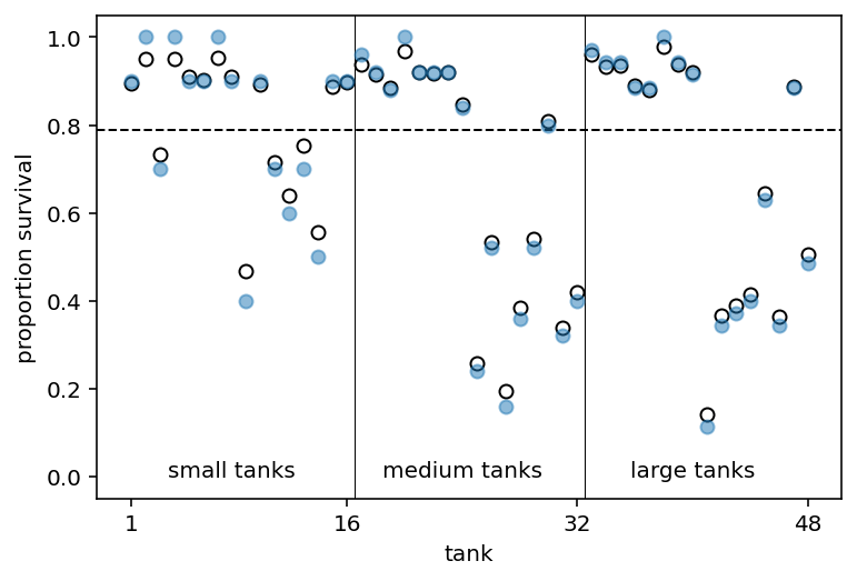
Here is how to read above plot -

• The dashed line locates the average proportion of survivors across all tanks

• The vertical lines divide tanks with different initial densities of tadpoles: small tanks (10 tad- poles), medium tanks (25), and large tanks (35).

• Empirical proportions of survivors in each tadpole tank, shown by the filled blue points, plotted with the 48 per-tank parameters from the multilevel model, shown by the black circles

In every tank, the posterior mean from the multilevel model is closer to the dashed line than the empir- ical proportion is.

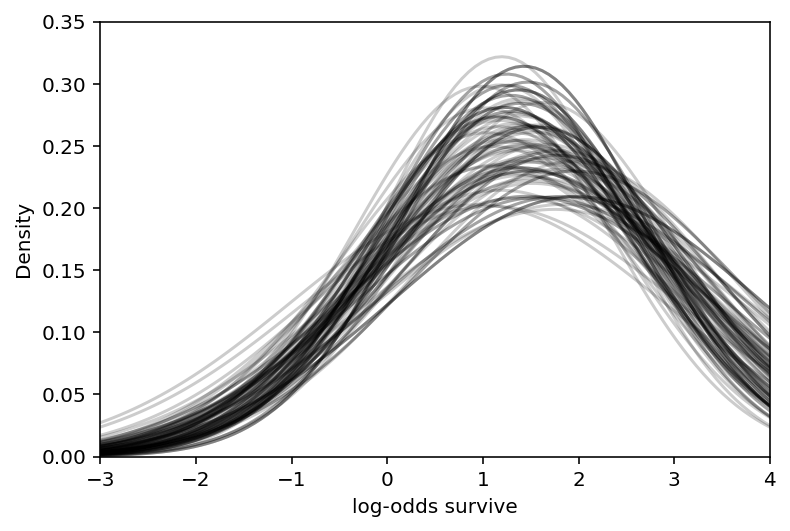
Code 13.6

sample_sigma = trace_13_2.posterior["sigma"].values[0]

# show first 100 populations in the posterior
plt.subplot(xlim=(-3, 4), ylim=(0, 0.35), xlabel="log-odds survive", ylabel="Density")
for i in range(100):
    x = np.linspace(-3, 4, 101)
    plt.plot(
        x,
        tf.exp(tfd.Normal(sample_a_bar[i], sample_sigma[i]).log_prob(x)),
        "k",
        alpha=0.2,
    )
plt.show()

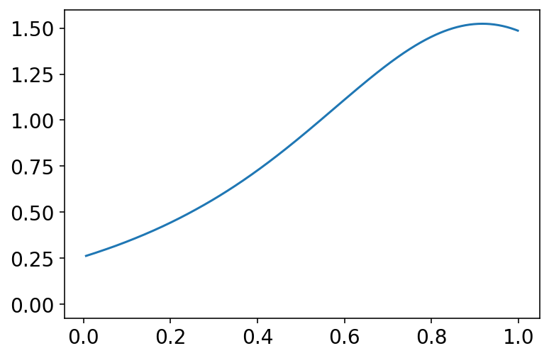
# sample 8000 imaginary tanks from the posterior distribution
idxs = np.random.randint(size=(8000,), low=0, high=499)

sim_tanks = tfd.Normal(sample_a_bar[idxs], sample_sigma[idxs]).sample()

# transform to probability and visualize
az.plot_kde(tf.sigmoid(sim_tanks).numpy(), bw=0.3)
plt.show()

13.2 Varying effects and the underlying/overfitting trade-off

13.2.1 The model

13.2.2 Assign values to the parameters

Code 13.7

a_bar = 1.5
sigma = 1.5
nponds = 60
Ni = np.repeat(np.array([5, 10, 25, 35]), repeats=15)

Code 13.8

a_pond = tfd.Normal(a_bar, sigma).sample((nponds,))

Code 13.9

dsim = pd.DataFrame(dict(pond=range(1, nponds + 1), Ni=Ni, true_a=a_pond))

dsim.describe()

	pond	Ni	true_a
count	60.000000	60.000000	60.000000
mean	30.500000	18.750000	1.800224
std	17.464249	12.024868	1.583633
min	1.000000	5.000000	-1.744786
25%	15.750000	8.750000	0.904637
50%	30.500000	17.500000	1.657137
75%	45.250000	27.500000	3.029984
max	60.000000	35.000000	5.816074

Code 13.10

print(type(range(3)))
print(type(np.arange(3)))

<class 'range'>
<class 'numpy.ndarray'>

13.2.3 Simulate survivors

Code 13.11

dsim["Si"] = tfd.Binomial(
    tf.cast(dsim.Ni.values, dtype=tf.float32), logits=dsim.true_a.values
).sample()

13.2.4 Compute the no-pooling estimates

Code 13.12

dsim["p_nopool"] = dsim.Si / dsim.Ni

13.2.5 Compute partial pooling estimates

Code 13.13

alpha_sample_shape = dsim.pond.shape[0]

dsim["pond_adj"] = dsim.pond.values - 1

tdf = dataframe_to_tensors(
    "SimulatedPonds",
    dsim,
    {"Si": tf.float32, "true_a": tf.float32, "Ni": tf.float32, "pond_adj": tf.int32},
)

def model_13_3(pid, N):
    def _generator():
        a_bar = yield Root(tfd.Sample(tfd.Normal(loc=0.0, scale=1.5), sample_shape=1))
        sigma = yield Root(tfd.Sample(tfd.Exponential(rate=1.0), sample_shape=1))
        alpha = yield tfd.Sample(
            tfd.Normal(loc=a_bar, scale=sigma), sample_shape=alpha_sample_shape
        )
        p = tf.sigmoid(tf.squeeze(tf.gather(alpha, pid, axis=-1)))

        Si = yield tfd.Independent(
            tfd.Binomial(total_count=N, probs=p), reinterpreted_batch_ndims=1
        )

    return tfd.JointDistributionCoroutine(_generator, validate_args=False)


jdc_13_3 = model_13_3(tdf.pond_adj, tdf.Ni)

NUM_CHAINS_FOR_13_3 = 2

init_state = [
    tf.zeros([NUM_CHAINS_FOR_13_3]),
    tf.ones([NUM_CHAINS_FOR_13_3]),
    tf.zeros([NUM_CHAINS_FOR_13_3, alpha_sample_shape]),
]

bijectors = [tfb.Identity(), tfb.Exp(), tfb.Identity()]

posterior_13_3, trace_13_3 = sample_posterior(
    jdc_13_3,
    observed_data=(tdf.Si,),
    params=["a_bar", "sigma", "alpha"],
    num_chains=NUM_CHAINS_FOR_13_3,
    init_state=init_state,
    bijectors=bijectors,
)

WARNING:tensorflow:@custom_gradient grad_fn has 'variables' in signature, but no ResourceVariables were used on the forward pass.

Code 13.14

az.summary(trace_13_3, round_to=2, kind="all", hdi_prob=0.89)

	mean	sd	hdi_5.5%	hdi_94.5%	mcse_mean	mcse_sd	ess_bulk	ess_tail	r_hat
a_bar	1.71	0.25	1.31	2.07	0.02	0.02	134.17	216.23	1.00
sigma	1.70	0.21	1.33	2.01	0.03	0.02	36.63	31.59	1.03
alpha[0]	-1.32	0.96	-2.98	0.06	0.14	0.10	48.28	139.86	1.03
alpha[1]	0.81	0.88	-0.71	2.12	0.11	0.08	66.09	113.68	1.01
alpha[2]	1.81	0.93	0.43	3.31	0.19	0.13	23.36	148.75	1.11
...	...	...	...	...	...	...	...	...	...
alpha[55]	0.97	0.36	0.38	1.48	0.02	0.01	336.63	464.41	1.00
alpha[56]	4.36	1.05	2.89	6.09	0.20	0.15	30.78	146.63	1.08
alpha[57]	2.13	0.52	1.48	3.13	0.04	0.03	186.25	330.32	1.00
alpha[58]	1.89	0.49	1.10	2.63	0.03	0.02	203.22	389.36	1.01
alpha[59]	2.38	0.59	1.54	3.29	0.06	0.04	104.91	189.12	1.02

62 rows × 9 columns

Code 13.15

sample_alpha = trace_13_3.posterior["alpha"].values[0]
dsim["p_partpool"] = tf.reduce_mean(tf.sigmoid(sample_alpha)).numpy()

Code 13.16

dsim["p_true"] = tf.sigmoid(dsim.true_a.values).numpy()

Code 13.17

nopool_error = (dsim.p_nopool - dsim.p_true).abs()
partpool_error = (dsim.p_partpool - dsim.p_true).abs()

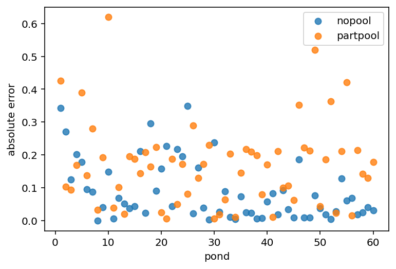
Code 13.18

plt.scatter(range(1, 61), nopool_error, label="nopool", alpha=0.8)
plt.gca().set(xlabel="pond", ylabel="absolute error")
plt.scatter(range(1, 61), partpool_error, label="partpool", alpha=0.8)
plt.legend()
plt.show()

Code 13.19

dsim["nopool_error"] = nopool_error
dsim["partpool_error"] = partpool_error
nopool_avg = dsim.groupby("Ni")["nopool_error"].mean()
partpool_avg = dsim.groupby("Ni")["partpool_error"].mean()

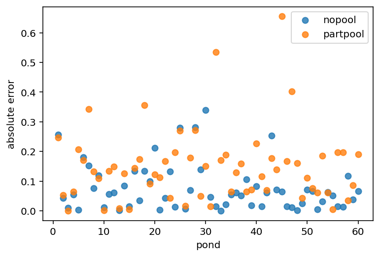
Overthiking: Repeating the pond simulation

Code 13.20

a_bar = 1.5
sigma = 1.5
nponds = 60
Ni = np.repeat(np.array([5, 10, 25, 35]), repeats=15)
a_pond = tfd.Normal(a_bar, sigma).sample((nponds,)).numpy()
dsim = pd.DataFrame(dict(pond=range(1, nponds + 1), Ni=Ni, true_a=a_pond))
dsim["Si"] = tfd.Binomial(
    tf.cast(dsim.Ni.values, dtype=tf.float32), logits=dsim.true_a.values
).sample()
dsim["p_nopool"] = dsim.Si / dsim.Ni

newdat = dict(
    Si=tf.cast(dsim.Si.values, dtype=tf.float32),
    Ni=tf.cast(dsim.Ni.values, dtype=tf.float32),
    pond=dsim.pond.values - 1,
)

jdc_13_3new = model_13_3(newdat["pond"], newdat["Ni"])

posterior_13_3new, trace_13_3new = sample_posterior(
    jdc_13_3new,
    observed_data=(newdat["Si"],),
    params=["a_bar", "sigma", "alpha"],
    num_chains=NUM_CHAINS_FOR_13_3,
    init_state=init_state,
    bijectors=bijectors,
)

sample_alpha = trace_13_3new.posterior["alpha"].values[0]
dsim["p_partpool"] = tf.reduce_mean(tf.sigmoid(sample_alpha)).numpy()
dsim["p_true"] = tf.sigmoid(dsim.true_a.values).numpy()
nopool_error = (dsim.p_nopool - dsim.p_true).abs()
partpool_error = (dsim.p_partpool - dsim.p_true).abs()
plt.scatter(range(1, 61), nopool_error, label="nopool", alpha=0.8)
plt.gca().set(xlabel="pond", ylabel="absolute error")
plt.scatter(range(1, 61), partpool_error, label="partpool", alpha=0.8)
plt.legend()
plt.show()

13.3 More than one type of cluster

13.3.1 Multilevel chimpanzees

Code 13.21

d = RethinkingDataset.Chimpanzees.get_dataset()

d["treatment"] = 1 + d.prosoc_left + 2 * d.condition - 1
d["block_id"] = d.block.values - 1
d["actor_id"] = d.actor.values - 1

tdf = dataframe_to_tensors(
    "Chimpanzee",
    d,
    {
        "treatment": tf.int32,
        "block_id": tf.int32,
        "actor_id": tf.int32,
        "pulled_left": tf.float32,
    },
)


def model_13_4(actor, block_id, treatment):
    def _generator():
        # hyper-priors
        a_bar = yield Root(tfd.Sample(tfd.Normal(loc=0.0, scale=1.5), sample_shape=1))
        sigma_a = yield Root(tfd.Sample(tfd.Exponential(rate=1.0), sample_shape=1))
        sigma_g = yield Root(tfd.Sample(tfd.Exponential(rate=1.0), sample_shape=1))
        # adaptive priors
        alpha = yield tfd.Sample(tfd.Normal(loc=a_bar, scale=sigma_a), sample_shape=7)
        gamma = yield tfd.Sample(tfd.Normal(loc=0.0, scale=sigma_g), sample_shape=6)
        beta = yield tfd.Sample(tfd.Normal(loc=0.0, scale=0.5), sample_shape=4)

        # three terms
        term1 = tf.squeeze(tf.gather(alpha, actor, axis=-1))
        term2 = tf.squeeze(tf.gather(gamma, block_id, axis=-1))
        term3 = tf.squeeze(tf.gather(beta, treatment, axis=-1))

        p = tf.sigmoid(term1 + term2 + term3)

        PL = yield tfd.Independent(
            tfd.Binomial(total_count=1, probs=p), reinterpreted_batch_ndims=1
        )

    return tfd.JointDistributionCoroutine(_generator, validate_args=False)


jdc_13_4 = model_13_4(tdf.actor_id, tdf.block_id, tdf.treatment)

NUM_CHAINS_FOR_13_4 = 2

init_state = [
    tf.zeros([NUM_CHAINS_FOR_13_4]),
    tf.ones([NUM_CHAINS_FOR_13_4]),
    tf.ones([NUM_CHAINS_FOR_13_4]),
    tf.zeros([NUM_CHAINS_FOR_13_4, 7]),
    tf.zeros([NUM_CHAINS_FOR_13_4, 6]),
    tf.zeros([NUM_CHAINS_FOR_13_4, 4]),
]

bijectors = [
    tfb.Identity(),
    tfb.Exp(),
    tfb.Exp(),
    tfb.Identity(),
    tfb.Identity(),
    tfb.Identity(),
]

posterior_13_4, trace_13_4 = sample_posterior(
    jdc_13_4,
    observed_data=(tdf.pulled_left,),
    params=["a_bar", "sigma_a", "sigma_g", "alpha", "gamma", "beta"],
    num_chains=NUM_CHAINS_FOR_13_4,
    init_state=init_state,
    bijectors=bijectors,
)

WARNING:tensorflow:@custom_gradient grad_fn has 'variables' in signature, but no ResourceVariables were used on the forward pass.

WARNING:tensorflow:5 out of the last 5 calls to <function run_hmc_chain at 0x7f425f530830> triggered tf.function retracing. Tracing is expensive and the excessive number of tracings could be due to (1) creating @tf.function repeatedly in a loop, (2) passing tensors with different shapes, (3) passing Python objects instead of tensors. For (1), please define your @tf.function outside of the loop. For (2), @tf.function has experimental_relax_shapes=True option that relaxes argument shapes that can avoid unnecessary retracing. For (3), please refer to https://www.tensorflow.org/guide/function#controlling_retracing and https://www.tensorflow.org/api_docs/python/tf/function for  more details.

Code 13.22

az.summary(trace_13_4, round_to=2, kind="all", hdi_prob=0.89)

	mean	sd	hdi_5.5%	hdi_94.5%	mcse_mean	mcse_sd	ess_bulk	ess_tail	r_hat
a_bar	0.37	0.69	-0.91	1.43	0.36	0.28	3.58	28.95	1.63
sigma_a	2.34	0.64	1.34	3.09	0.11	0.08	29.31	102.41	1.08
sigma_g	0.16	0.12	0.03	0.35	0.04	0.03	7.07	5.64	1.22
alpha[0]	-0.42	0.34	-0.92	0.15	0.14	0.11	5.63	48.11	1.31
alpha[1]	5.80	1.19	3.63	7.48	0.66	0.52	3.26	15.06	1.67
alpha[2]	-0.76	0.36	-1.39	-0.31	0.14	0.10	6.50	31.89	1.24
alpha[3]	-0.79	0.37	-1.28	-0.16	0.15	0.11	6.34	95.57	1.25
alpha[4]	-0.46	0.33	-0.99	0.03	0.11	0.08	8.42	77.27	1.17
alpha[5]	0.50	0.35	-0.00	1.10	0.12	0.09	8.99	118.84	1.18
alpha[6]	2.00	0.45	1.40	2.82	0.18	0.14	6.73	22.86	1.23
gamma[0]	-0.15	0.20	-0.51	0.09	0.06	0.04	18.13	165.90	1.08
gamma[1]	0.03	0.17	-0.17	0.35	0.02	0.02	86.82	26.03	1.12
gamma[2]	0.05	0.15	-0.12	0.30	0.01	0.01	219.86	196.90	1.05
gamma[3]	0.02	0.14	-0.24	0.21	0.01	0.02	210.41	221.32	1.16
gamma[4]	-0.02	0.13	-0.23	0.20	0.01	0.02	238.49	189.11	1.06
gamma[5]	0.09	0.16	-0.15	0.37	0.02	0.02	164.11	119.75	1.03
beta[0]	-0.08	0.30	-0.55	0.35	0.11	0.08	6.95	144.63	1.23
beta[1]	0.46	0.30	-0.06	0.92	0.12	0.09	5.57	41.29	1.29
beta[2]	-0.41	0.28	-0.84	0.08	0.12	0.09	5.94	62.42	1.26
beta[3]	0.40	0.31	-0.11	0.83	0.11	0.08	8.06	48.98	1.20

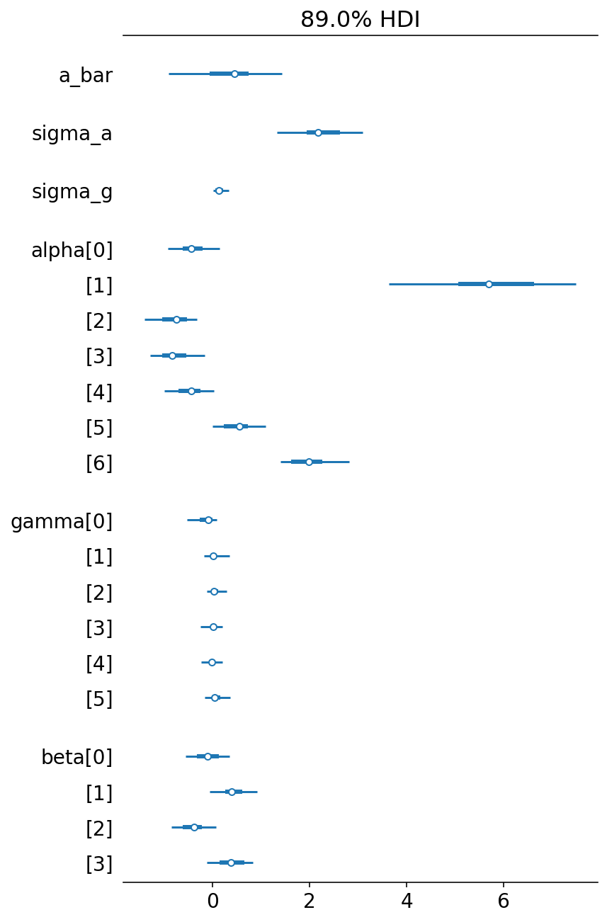
Note that there is variation across parameters when it comes to effective sample size (ess_mean). This is because some parameters spends a lot of time near a boundary.

az.plot_forest(trace_13_4, combined=True, hdi_prob=0.89)
plt.show()

Code 13.23

Build a model that ignores block so that we can then compare it with the above model

def model_13_5(actor, treatment):
    def _generator():
        # hyper-priors
        a_bar = yield Root(tfd.Sample(tfd.Normal(loc=0.0, scale=1.5), sample_shape=1))
        sigma_a = yield Root(tfd.Sample(tfd.Exponential(rate=1.0), sample_shape=1))
        # adaptive priors
        alpha = yield tfd.Sample(tfd.Normal(loc=a_bar, scale=sigma_a), sample_shape=7)
        beta = yield tfd.Sample(tfd.Normal(loc=0.0, scale=0.5), sample_shape=4)

        # two terms
        term1 = tf.squeeze(tf.gather(alpha, actor, axis=-1))
        term2 = tf.squeeze(tf.gather(beta, treatment, axis=-1))

        p = tf.sigmoid(term1 + term2)

        PL = yield tfd.Independent(
            tfd.Binomial(total_count=1, probs=p), reinterpreted_batch_ndims=1
        )

    return tfd.JointDistributionCoroutine(_generator, validate_args=False)


jdc_13_5 = model_13_5(tdf.actor_id, tdf.treatment)


NUM_CHAINS_FOR_13_5 = 2

init_state = [
    tf.zeros([NUM_CHAINS_FOR_13_5]),
    tf.ones([NUM_CHAINS_FOR_13_5]),
    tf.zeros([NUM_CHAINS_FOR_13_5, 7]),
    tf.zeros([NUM_CHAINS_FOR_13_5, 4]),
]

bijectors = [tfb.Identity(), tfb.Exp(), tfb.Identity(), tfb.Identity()]

posterior_13_5, trace_13_5 = sample_posterior(
    jdc_13_5,
    observed_data=(tdf.pulled_left,),
    params=["a_bar", "sigma_a", "alpha", "beta"],
    num_chains=NUM_CHAINS_FOR_13_5,
    init_state=init_state,
    bijectors=bijectors,
)

WARNING:tensorflow:6 out of the last 6 calls to <function run_hmc_chain at 0x7f425f530830> triggered tf.function retracing. Tracing is expensive and the excessive number of tracings could be due to (1) creating @tf.function repeatedly in a loop, (2) passing tensors with different shapes, (3) passing Python objects instead of tensors. For (1), please define your @tf.function outside of the loop. For (2), @tf.function has experimental_relax_shapes=True option that relaxes argument shapes that can avoid unnecessary retracing. For (3), please refer to https://www.tensorflow.org/guide/function#controlling_retracing and https://www.tensorflow.org/api_docs/python/tf/function for  more details.

Code 13.24

def compute_and_store_log_likelihood_for_model_13_4():

    sample_a_bar = posterior_13_4["a_bar"]
    sample_sigma_a = posterior_13_4["sigma_a"]
    sample_sigma_g = posterior_13_4["sigma_g"]

    sample_alpha = posterior_13_4["alpha"]
    sample_gamma = posterior_13_4["gamma"]
    sample_beta = posterior_13_4["beta"]

    ds, _ = jdc_13_4.sample_distributions(
        value=[
            sample_a_bar,
            sample_sigma_a,
            sample_sigma_g,
            sample_alpha,
            sample_gamma,
            sample_beta,
            None,
        ]
    )

    log_likelihood_13_4 = ds[-1].distribution.log_prob(tdf.pulled_left).numpy()

    # we need to insert this in the sampler_stats
    sample_stats_13_4 = trace_13_4.sample_stats

    coords = [
        sample_stats_13_4.coords["chain"],
        sample_stats_13_4.coords["draw"],
        np.arange(504),
    ]

    sample_stats_13_4["log_likelihood"] = xr.DataArray(
        log_likelihood_13_4,
        coords=coords,
        dims=["chain", "draw", "log_likelihood_dim_0"],
    )


compute_and_store_log_likelihood_for_model_13_4()

def compute_and_store_log_likelihood_for_model_13_5():

    sample_a_bar = posterior_13_5["a_bar"]
    sample_sigma_a = posterior_13_5["sigma_a"]

    sample_alpha = posterior_13_5["alpha"]
    sample_beta = posterior_13_5["beta"]

    ds, _ = jdc_13_5.sample_distributions(
        value=[sample_a_bar, sample_sigma_a, sample_alpha, sample_beta, None]
    )

    log_likelihood_13_5 = ds[-1].distribution.log_prob(tdf.pulled_left).numpy()

    # we need to insert this in the sampler_stats
    sample_stats_13_5 = trace_13_5.sample_stats

    coords = [
        sample_stats_13_5.coords["chain"],
        sample_stats_13_5.coords["draw"],
        np.arange(504),
    ]

    sample_stats_13_5["log_likelihood"] = xr.DataArray(
        log_likelihood_13_5,
        coords=coords,
        dims=["chain", "draw", "log_likelihood_dim_0"],
    )


compute_and_store_log_likelihood_for_model_13_5()

az.compare({"m13.4": trace_13_4, "m13.5": trace_13_5})

/opt/hostedtoolcache/Python/3.7.12/x64/lib/python3.7/site-packages/arviz/stats/stats.py:695: UserWarning: Estimated shape parameter of Pareto distribution is greater than 0.7 for one or more samples. You should consider using a more robust model, this is because importance sampling is less likely to work well if the marginal posterior and LOO posterior are very different. This is more likely to happen with a non-robust model and highly influential observations.
  "Estimated shape parameter of Pareto distribution is greater than 0.7 for "

	rank	loo	p_loo	d_loo	weight	se	dse	warning	loo_scale
m13.4	0	-265.148032	10.345738	0.000000	1.000000e+00	9.724156	0.000000	True	log
m13.5	1	-268.657733	11.521361	3.509701	7.549517e-15	9.760426	0.858991	False	log

Above 2 models seem to imply nearly identical predictions. Should we select m13.4 as it is simpler among the two ?. Author here suggests that to select a model, we should rather want to test conditional independencies of different causal models.

13.3.2 Even more clusters

Code 13.25

m13.4 with partial pooling on the treatments

def model_13_6(actor, block_id, treatment):
    def _generator():
        # hyper-priors
        a_bar = yield Root(tfd.Sample(tfd.Normal(loc=0.0, scale=1.5), sample_shape=1))
        sigma_a = yield Root(tfd.Sample(tfd.Exponential(rate=1.0), sample_shape=1))
        sigma_g = yield Root(tfd.Sample(tfd.Exponential(rate=1.0), sample_shape=1))
        sigma_b = yield Root(tfd.Sample(tfd.Exponential(rate=1.0), sample_shape=1))
        # adaptive priors
        alpha = yield tfd.Sample(tfd.Normal(loc=a_bar, scale=sigma_a), sample_shape=7)
        gamma = yield tfd.Sample(tfd.Normal(loc=0.0, scale=sigma_g), sample_shape=6)
        beta = yield tfd.Sample(tfd.Normal(loc=0.0, scale=sigma_b), sample_shape=4)

        # three terms
        term1 = tf.squeeze(tf.gather(alpha, actor, axis=-1))
        term2 = tf.squeeze(tf.gather(gamma, block_id, axis=-1))
        term3 = tf.squeeze(tf.gather(beta, treatment, axis=-1))

        p = tf.sigmoid(term1 + term2 + term3)

        PL = yield tfd.Independent(
            tfd.Binomial(total_count=1, probs=p), reinterpreted_batch_ndims=1
        )

    return tfd.JointDistributionCoroutine(_generator, validate_args=False)


jdc_13_6 = model_13_6(tdf.actor_id, tdf.block_id, tdf.treatment)

NUM_CHAINS_FOR_13_6 = 2

init_state = [
    tf.zeros([NUM_CHAINS_FOR_13_6]),
    tf.ones([NUM_CHAINS_FOR_13_6]),
    tf.ones([NUM_CHAINS_FOR_13_6]),
    tf.ones([NUM_CHAINS_FOR_13_6]),
    tf.zeros([NUM_CHAINS_FOR_13_6, 7]),
    tf.zeros([NUM_CHAINS_FOR_13_6, 6]),
    tf.zeros([NUM_CHAINS_FOR_13_6, 4]),
]

bijectors = [
    tfb.Identity(),
    tfb.Exp(),
    tfb.Exp(),
    tfb.Exp(),
    tfb.Identity(),
    tfb.Identity(),
    tfb.Identity(),
]

posterior_13_6, trace_13_6 = sample_posterior(
    jdc_13_6,
    observed_data=(tdf.pulled_left,),
    params=["a_bar", "sigma_a", "sigma_g", "sigma_b", "alpha", "gamma", "beta"],
    num_chains=NUM_CHAINS_FOR_13_6,
    init_state=init_state,
    bijectors=bijectors,
)

{
    "m13.4": np.mean(trace_13_4.posterior["beta"].values[1], 0),
    "m13.6": np.mean(trace_13_6.posterior["beta"].values[1], 0),
}

{'m13.4': array([-0.23599166,  0.30075985, -0.52458525,  0.32245275], dtype=float32),
 'm13.6': array([-0.09813196,  0.32820734, -0.39110982,  0.26330954], dtype=float32)}

13.4 Divergent transitions and non-centered priors

13.4.1 The Devil’s Funnel

Code 13.26 (TODO - add notes on divergence)

def model_13_7():
    def _generator():
        v = yield Root(tfd.Sample(tfd.Normal(loc=0.0, scale=3.0), sample_shape=1))
        x = yield tfd.Sample(tfd.Normal(loc=0.0, scale=tf.exp(v)), sample_shape=1)

    return tfd.JointDistributionCoroutine(_generator, validate_args=False)


jdc_13_7 = model_13_7()

NUM_CHAINS_FOR_13_7 = 2

init_state = [tf.zeros([NUM_CHAINS_FOR_13_7]), tf.zeros([NUM_CHAINS_FOR_13_7])]

bijectors = [tfb.Identity(), tfb.Identity()]

posterior_13_7, trace_13_7 = sample_posterior(
    jdc_13_7,
    observed_data=(),
    params=["v", "x"],
    num_chains=NUM_CHAINS_FOR_13_7,
    init_state=init_state,
    bijectors=bijectors,
)

az.summary(trace_13_7, hdi_prob=0.89)

	mean	sd	hdi_5.5%	hdi_94.5%	mcse_mean	mcse_sd	ess_bulk	ess_tail	r_hat
v	-1.658	0.967	-2.623	-0.581	0.678	0.573	2.0	2.0	3.37
x	0.521	0.427	0.094	0.969	0.299	0.253	3.0	2.0	2.25

Code 13.27

def model_13_7nc():
    def _generator():
        v = yield Root(tfd.Sample(tfd.Normal(loc=0.0, scale=3.0), sample_shape=1))
        z = yield Root(tfd.Sample(tfd.Normal(loc=0.0, scale=1.0), sample_shape=1))
        x = z * tf.exp(v)

    return tfd.JointDistributionCoroutine(_generator, validate_args=False)


jdc_13_7nc = model_13_7nc()

NUM_CHAINS_FOR_13_7nc = 2

init_state = [tf.zeros([NUM_CHAINS_FOR_13_7nc]), tf.zeros([NUM_CHAINS_FOR_13_7nc])]

bijectors = [tfb.Identity(), tfb.Identity()]

posterior_13_7nc, trace_13_7nc = sample_posterior(
    jdc_13_7nc,
    observed_data=(),
    params=["v", "z"],
    num_chains=NUM_CHAINS_FOR_13_7nc,
    init_state=init_state,
    bijectors=bijectors,
)

az.summary(trace_13_7nc, hdi_prob=0.89)

	mean	sd	hdi_5.5%	hdi_94.5%	mcse_mean	mcse_sd	ess_bulk	ess_tail	r_hat
v	-0.027	2.945	-5.198	4.307	0.076	0.093	1480.0	705.0	1.00
z	0.034	0.991	-1.554	1.494	0.121	0.086	68.0	235.0	1.04

13.4.2 Non-centered chimpanzees

Code 13.28 [TODO - parameterize the target accept prob]

Code 13.29

def model_13_4nc(actor, block_id, treatment):
    def _generator():
        # hyper-priors
        a_bar = yield Root(tfd.Sample(tfd.Normal(loc=0.0, scale=1.5), sample_shape=1))
        sigma_a = yield Root(tfd.Sample(tfd.Exponential(rate=1.0), sample_shape=1))
        sigma_g = yield Root(tfd.Sample(tfd.Exponential(rate=1.0), sample_shape=1))
        # adaptive priors
        z = yield tfd.Sample(tfd.Normal(loc=0.0, scale=1.0), sample_shape=7)
        x = yield tfd.Sample(tfd.Normal(loc=0.0, scale=1.0), sample_shape=6)
        b = yield tfd.Sample(tfd.Normal(loc=0.0, scale=0.5), sample_shape=4)

        # three terms
        term1 = tf.squeeze(tf.gather(z, actor, axis=-1))
        term2 = tf.squeeze(tf.gather(x, block_id, axis=-1))
        term3 = tf.squeeze(tf.gather(b, treatment, axis=-1))

        # reparamertization
        r = (
            a_bar[..., tf.newaxis]
            + sigma_a[..., tf.newaxis] * term1
            + sigma_g[..., tf.newaxis] * term2
            + term3
        )

        p = tf.sigmoid(r)

        PL = yield tfd.Independent(
            tfd.Binomial(total_count=1, probs=p), reinterpreted_batch_ndims=1
        )

    return tfd.JointDistributionCoroutine(_generator, validate_args=False)


jdc_13_4nc = model_13_4nc(tdf.actor_id, tdf.block_id, tdf.treatment)

s = jdc_13_4nc.sample(2)

jdc_13_4nc.log_prob(s)

WARNING:tensorflow:5 out of the last 11 calls to <function _random_binomial at 0x7f425fd90200> triggered tf.function retracing. Tracing is expensive and the excessive number of tracings could be due to (1) creating @tf.function repeatedly in a loop, (2) passing tensors with different shapes, (3) passing Python objects instead of tensors. For (1), please define your @tf.function outside of the loop. For (2), @tf.function has experimental_relax_shapes=True option that relaxes argument shapes that can avoid unnecessary retracing. For (3), please refer to https://www.tensorflow.org/guide/function#controlling_retracing and https://www.tensorflow.org/api_docs/python/tf/function for  more details.

WARNING:tensorflow:@custom_gradient grad_fn has 'variables' in signature, but no ResourceVariables were used on the forward pass.

<tf.Tensor: shape=(2, 2), dtype=float32, numpy=
array([[-146.41957, -147.74915],
       [-164.2373 , -165.5669 ]], dtype=float32)>

NUM_CHAINS_FOR_13_4 = 2

init_state = [
    tf.zeros([NUM_CHAINS_FOR_13_4]),
    tf.ones([NUM_CHAINS_FOR_13_4]),
    tf.ones([NUM_CHAINS_FOR_13_4]),
    tf.zeros([NUM_CHAINS_FOR_13_4, 7]),
    tf.zeros([NUM_CHAINS_FOR_13_4, 6]),
    tf.zeros([NUM_CHAINS_FOR_13_4, 4]),
]

bijectors = [
    tfb.Identity(),
    tfb.Exp(),
    tfb.Exp(),
    tfb.Identity(),
    tfb.Identity(),
    tfb.Identity(),
]

posterior_13_4nc, trace_13_4nc = sample_posterior(
    jdc_13_4nc,
    observed_data=(tdf.pulled_left,),
    params=["a_bar", "sigma_a", "sigma_g", "z", "x", "b"],
    num_chains=NUM_CHAINS_FOR_13_4,
    init_state=init_state,
    bijectors=bijectors,
)

az.summary(trace_13_4nc, hdi_prob=0.89)

	mean	sd	hdi_5.5%	hdi_94.5%	mcse_mean	mcse_sd	ess_bulk	ess_tail	r_hat
a_bar	0.718	0.597	-0.198	1.656	0.095	0.072	40.0	39.0	1.03
sigma_a	1.966	0.541	1.122	2.752	0.119	0.086	23.0	165.0	1.08
sigma_g	0.199	0.146	0.005	0.382	0.064	0.048	4.0	37.0	1.45
z[0]	-0.539	0.297	-0.999	-0.104	0.038	0.027	58.0	131.0	1.03
z[1]	2.118	0.541	1.281	2.964	0.105	0.075	23.0	47.0	1.08
z[2]	-0.718	0.336	-1.190	-0.188	0.047	0.033	51.0	100.0	1.03
z[3]	-0.718	0.328	-1.219	-0.216	0.045	0.032	51.0	95.0	1.04
z[4]	-0.558	0.310	-0.998	-0.024	0.042	0.030	54.0	93.0	1.02
z[5]	-0.044	0.303	-0.460	0.489	0.039	0.027	62.0	120.0	1.03
z[6]	0.781	0.405	0.127	1.335	0.053	0.038	56.0	52.0	1.06
x[0]	-0.710	1.079	-2.232	0.965	0.527	0.402	4.0	21.0	1.42
x[1]	0.176	0.851	-1.230	1.426	0.261	0.190	11.0	53.0	1.18
x[2]	0.424	0.721	-0.746	1.557	0.124	0.089	34.0	104.0	1.09
x[3]	-0.208	0.813	-1.467	1.133	0.419	0.323	4.0	34.0	1.52
x[4]	-0.242	0.806	-1.518	1.094	0.148	0.173	30.0	29.0	1.10
x[5]	0.458	0.889	-0.794	1.896	0.428	0.326	5.0	118.0	1.40
b[0]	-0.144	0.270	-0.575	0.289	0.034	0.024	63.0	252.0	1.02
b[1]	0.373	0.276	-0.000	0.879	0.030	0.022	83.0	227.0	1.03
b[2]	-0.494	0.281	-0.916	-0.026	0.036	0.026	59.0	122.0	1.01
b[3]	0.245	0.276	-0.125	0.729	0.038	0.027	54.0	171.0	1.02

Code 13.30 [TODO - do not how to compute ess]

13.5 Multilevel posterior predictions

13.5.1 Posterior prediction for same clusters

Code 13.31

chimp = 2
d_pred = dict(
    actor=np.repeat(chimp, 4) - 1, treatment=np.arange(4), block_id=np.repeat(1, 4) - 1
)

# we want to calculate the p using the posterior

sample_alpha = posterior_13_4["alpha"][0]
sample_gamma = posterior_13_4["gamma"][0]
sample_beta = posterior_13_4["beta"][0]

term1 = tf.squeeze(tf.gather(sample_alpha, d_pred["actor"], axis=-1))
term2 = tf.squeeze(tf.gather(sample_gamma, d_pred["block_id"], axis=-1))
term3 = tf.squeeze(tf.gather(sample_beta, d_pred["treatment"], axis=-1))

p = tf.sigmoid(term1 + term2 + term3)

p_mu = tf.reduce_mean(p, 0)
p_ci = tfp.stats.percentile(p, q=(5.5, 94.5), axis=0)

p_mu, p_ci

(<tf.Tensor: shape=(4,), dtype=float32, numpy=array([0.9902569 , 0.9942323 , 0.98575664, 0.99342287], dtype=float32)>,
 <tf.Tensor: shape=(2, 4), dtype=float32, numpy=
 array([[0.96957153, 0.9826287 , 0.9497617 , 0.9785687 ],
        [0.9995152 , 0.9997659 , 0.99941087, 0.9997306 ]], dtype=float32)>)

Code 13.32

{k: v.values[0].reshape(-1)[:5] for k, v in trace_13_4.posterior.items()}

{'a_bar': array([-0.09083581, -0.01601001, -0.01601001,  0.30656427,  0.00250988],
       dtype=float32),
 'sigma_a': array([1.773968 , 1.8867178, 1.8867178, 1.2840902, 1.6988628],
       dtype=float32),
 'sigma_g': array([0.1504367 , 0.16048822, 0.16048822, 0.15172496, 0.16895404],
       dtype=float32),
 'alpha': array([-0.53260475,  4.149923  , -0.6222214 , -0.7914526 , -0.60494405],
       dtype=float32),
 'gamma': array([-0.14206514,  0.21386218, -0.00097559,  0.2273949 , -0.07356969],
       dtype=float32),
 'beta': array([ 0.0456219 ,  0.6748041 , -0.06900286,  0.39875892, -0.08693071],
       dtype=float32)}

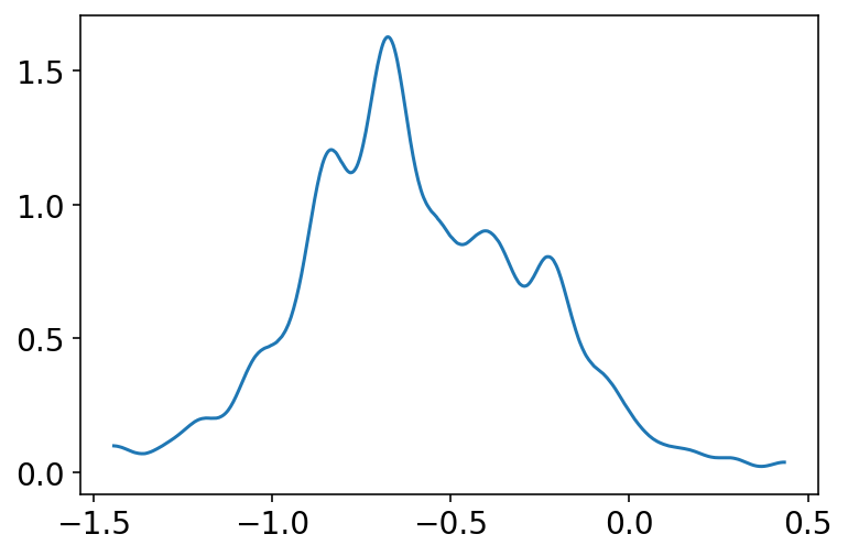
Code 13.33

az.plot_kde(trace_13_4.posterior["alpha"].values[0][:, 4])
plt.show()

Code 13.34

post = trace_13_4.posterior

def p_link(treatment, actor=0, block_id=0):
    a, g, b = post["alpha"].values[0], post["gamma"].values[0], post["beta"].values[0]
    logodds = a[:, actor] + g[:, block_id] + b[:, treatment]
    return tf.sigmoid(logodds)

Code 13.35

p_raw = list(map(lambda i: p_link(i, actor=1, block_id=0), np.arange(4)))
p_mu = np.mean(p_raw, 0)
p_ci = np.percentile(p_raw, (5.5, 94.5), 0)

13.5.2 Posterior prediction for new clusters

Code 13.36

def p_link_abar(treatment):
    logodds = post["a_bar"].values[0] + post["beta"].values[0][:, treatment]
    return tf.sigmoid(logodds)

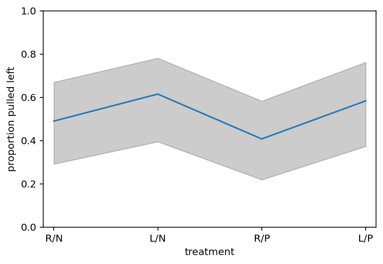
Code 13.37

p_raw = list(map(p_link_abar, np.arange(4)))
p_mu = np.mean(p_raw, 1)
p_ci = np.percentile(p_raw, (5.5, 94.5), 1)

plt.subplot(
    xlabel="treatment", ylabel="proportion pulled left", ylim=(0, 1), xlim=(0.9, 4.1)
)
plt.gca().set(xticks=range(1, 5), xticklabels=["R/N", "L/N", "R/P", "L/P"])
plt.plot(range(1, 5), p_mu)
plt.fill_between(range(1, 5), p_ci[0], p_ci[1], color="k", alpha=0.2)
plt.show()

Code 13.38

a_sim = tfd.Normal(
    loc=post["a_bar"].values[0], scale=post["sigma_a"].values[0]
).sample()


def p_link_asim(treatment):
    logodds = a_sim + post["beta"].values[0][:, treatment]
    return tf.sigmoid(logodds)


p_raw_asim = np.array(list(map(p_link_asim, np.arange(4))))

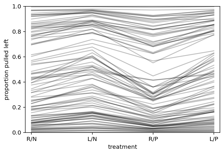
Code 13.39

plt.subplot(
    xlabel="treatment", ylabel="proportion pulled left", ylim=(0, 1), xlim=(0.9, 4.1)
)
plt.gca().set(xticks=range(1, 5), xticklabels=["R/N", "L/N", "R/P", "L/P"])
for i in range(100):
    plt.plot(range(1, 5), p_raw_asim[:, i], color="k", alpha=0.25)

previous

12. Monsters and Mixtures

next

14. Adventures in Covariance