6. The Haunted DAG and The Causal Terror
Contents
![]()
6. The Haunted DAG and The Causal Terror
# Install packages that are not installed in colab
try:
  import google.colab
  %pip install --upgrade -q daft
  %pip install -q causalgraphicalmodels
  %pip install -q watermark
  %pip install git+https://github.com/ksachdeva/rethinking-tensorflow-probability.git
except:
  pass
%load_ext watermark
# Core
import numpy as np
import arviz as az
import pandas as pd
import tensorflow as tf
import tensorflow_probability as tfp
from statsmodels.regression import linear_model

# visualization
import matplotlib.pyplot as plt

import daft
from causalgraphicalmodels import CausalGraphicalModel

from rethinking.data import RethinkingDataset
from rethinking.data import dataframe_to_tensors
from rethinking.mcmc import sample_posterior

# aliases
tfd = tfp.distributions
tfb = tfp.bijectors
Root = tfd.JointDistributionCoroutine.Root
2022-01-19 18:56:08.883549: W tensorflow/stream_executor/platform/default/dso_loader.cc:64] Could not load dynamic library 'libcudart.so.11.0'; dlerror: libcudart.so.11.0: cannot open shared object file: No such file or directory
2022-01-19 18:56:08.883587: I tensorflow/stream_executor/cuda/cudart_stub.cc:29] Ignore above cudart dlerror if you do not have a GPU set up on your machine.
%watermark -p numpy,tensorflow,tensorflow_probability,arviz,scipy,pandas,statsmodels,daft,causalgraphicalmodels,rethinking
numpy                 : 1.21.5
tensorflow            : 2.7.0
tensorflow_probability: 0.15.0
arviz                 : 0.11.4
scipy                 : 1.7.3
pandas                : 1.3.5
statsmodels           : 0.13.1
daft                  : 0.1.2
causalgraphicalmodels : 0.0.4
rethinking            : 0.1.0
# config of various plotting libraries
%config InlineBackend.figure_format = 'retina'
Berkson’s paradox - A false observation of a negative coorelation between 2 positive traits.
Members of a population which have some positive trait tend to lack a second even though -:
The traits may be unrelated
Or, they may be even positively related.
e.g Resturants at good location have bad food even though location & food have no correlation
Berkon’s paradox is also called selection-distortion effect.
The gist of the idea here is that when a sample is selected on a combination of 2 (or more) variables, the relationship between those 2 variables is different after selection than it was before.
Because of above, we should always be cautious of adding more predictor variables to our regression as it may introduce statistical selection with in the model. The phenomenon has a name and it is called COLLIDER BIAS.
There are actually 3 types of hazards when we add more predictor variables -
Multicollinearity
Post treatment bias
Collider bias
Collider - a beam in which two particles are made to collide (collision)
Overthinking : Simulated Science Distorion
Code 6.1
A simulated example to demonstrate selection-distortion effect. It has been observed that newsworthiness and trustworthiness of papers accepted by journal are factors in getting the funding.
Below code shows how they correlated with each other.
# A simulated example to demonstrate selection-disortion
#
# Here

_SEED = 1914

N = 200
p = 0.1  # proportion to select

# uncorrelated newsworthiness & trustworthiness
seed = tfp.util.SeedStream(_SEED, salt="")
nw = tfd.Normal(loc=0.0, scale=1.0).sample(N, seed=seed()).numpy()
seed = tfp.util.SeedStream(_SEED, salt="")
tw = tfd.Normal(loc=0.0, scale=1.0).sample(N, seed=seed()).numpy()

# select top 10% of combined scores
s = nw + tw  # total score
q = np.quantile(s, 1 - p)  # top 10% threshold

selected = np.where(s >= q, True, False)

np.corrcoef(tw[selected], nw[selected])[0, 1]
2022-01-19 18:56:11.517832: W tensorflow/stream_executor/platform/default/dso_loader.cc:64] Could not load dynamic library 'libcuda.so.1'; dlerror: libcuda.so.1: cannot open shared object file: No such file or directory
2022-01-19 18:56:11.517869: W tensorflow/stream_executor/cuda/cuda_driver.cc:269] failed call to cuInit: UNKNOWN ERROR (303)
2022-01-19 18:56:11.517894: I tensorflow/stream_executor/cuda/cuda_diagnostics.cc:156] kernel driver does not appear to be running on this host (fv-az272-145): /proc/driver/nvidia/version does not exist
2022-01-19 18:56:11.519166: I tensorflow/core/platform/cpu_feature_guard.cc:151] This TensorFlow binary is optimized with oneAPI Deep Neural Network Library (oneDNN) to use the following CPU instructions in performance-critical operations:  AVX2 FMA
To enable them in other operations, rebuild TensorFlow with the appropriate compiler flags.
-0.828225254885134
This shows that nw (newsworthiness) & tw (trustworthiness) are heavily negivately correlated.
6.1 Multicollinearity
Multicollinearity happens when the predictor variables are stronly correlated.
When this happens the posterior distribution will seem to suggest that none of the variables is reliably associated with the outcome.
Model will still infer correct results but it would be difficult to understand it.
6.1.1 Multicollinear legs
Here we create an artifical dataset about height & its relation to the length of the legs as predictor variables.
The two legs are more or less of same length so they are correlated with each other. Including both of the legs as the predictors result in multicollinearity
Code 6.2
_SEED = 909

N = 100


def generate_height_leg_data():
    seed = tfp.util.SeedStream(_SEED, salt="leg_exp")
    height = tfd.Normal(loc=10.0, scale=2.0).sample(N, seed=seed()).numpy()
    leg_prop = tfd.Uniform(low=0.4, high=0.5).sample(N, seed=seed()).numpy()

    # left & right leg as proportion + error
    leg_left = (
        leg_prop * height + tfd.Normal(loc=0, scale=0.02).sample(N, seed=seed()).numpy()
    )

    leg_right = (
        leg_prop * height + tfd.Normal(loc=0, scale=0.02).sample(N, seed=seed()).numpy()
    )

    # build a dataframe using above
    d = pd.DataFrame({"height": height, "leg_left": leg_left, "leg_right": leg_right})

    return d


d = generate_height_leg_data()

d.describe()
| height | leg_left | leg_right | |
|---|---|---|---|
| count | 100.000000 | 100.000000 | 100.000000 |
| mean | 10.244188 | 4.586804 | 4.589090 |
| std | 1.971723 | 0.856999 | 0.857432 |
| min | 6.569585 | 2.711091 | 2.734310 |
| 25% | 8.705090 | 3.959075 | 3.970327 |
| 50% | 10.478082 | 4.628943 | 4.644671 |
| 75% | 11.372977 | 5.143220 | 5.147640 |
| max | 15.219750 | 7.189007 | 7.178730 |
Code 6.3
Very vague and bad priors are used in the model here so that we can be sure that priors are not responsible for what we are about to observe
tdf = dataframe_to_tensors("SimulatedHeight", d, ["leg_left", "leg_right", "height"])


def model_6_1(leg_left_data, leg_right_data):
    def _generator():
        alpha = yield Root(
            tfd.Sample(tfd.Normal(loc=10.0, scale=100.0, name="alpha"), sample_shape=1)
        )
        betaL = yield Root(
            tfd.Sample(tfd.Normal(loc=2.0, scale=10.0, name="betaL"), sample_shape=1)
        )
        betaR = yield Root(
            tfd.Sample(tfd.Normal(loc=2.0, scale=10.0, name="betaR"), sample_shape=1)
        )
        sigma = yield Root(
            tfd.Sample(tfd.Exponential(rate=1.0, name="sigma"), sample_shape=1)
        )

        mu = tf.squeeze(
            alpha[..., tf.newaxis]
            + betaL[..., tf.newaxis] * leg_left_data
            + betaR[..., tf.newaxis] * leg_right_data
        )

        scale = sigma[..., tf.newaxis]

        height = yield tfd.Independent(
            tfd.Normal(loc=mu, scale=scale, name="height"), reinterpreted_batch_ndims=1
        )

    return tfd.JointDistributionCoroutine(_generator, validate_args=False)


jdc_6_1 = model_6_1(tdf.leg_left, tdf.leg_right)
NUM_CHAINS_FOR_6_1 = 2

# Note -
# I got somewhat ok looking results with this init values
init_state = [
    tf.ones([NUM_CHAINS_FOR_6_1]),
    tf.ones([NUM_CHAINS_FOR_6_1]),
    tf.ones([NUM_CHAINS_FOR_6_1]),
    tf.ones([NUM_CHAINS_FOR_6_1]),
]

bijectors = [tfb.Identity(), tfb.Identity(), tfb.Identity(), tfb.Exp()]

observed_data = (tdf.height,)

posterior_6_1, trace_6_1 = sample_posterior(
    jdc_6_1,
    observed_data=observed_data,
    num_chains=NUM_CHAINS_FOR_6_1,
    init_state=init_state,
    bijectors=bijectors,
    num_samples=4000,
    burnin=500,
    params=["alpha", "betaL", "betaR", "sigma"],
)

az.summary(trace_6_1, hdi_prob=0.89)
| mean | sd | hdi_5.5% | hdi_94.5% | mcse_mean | mcse_sd | ess_bulk | ess_tail | r_hat | |
|---|---|---|---|---|---|---|---|---|---|
| alpha | 0.340 | 0.380 | -0.182 | 0.978 | 0.059 | 0.042 | 47.0 | 60.0 | 1.05 |
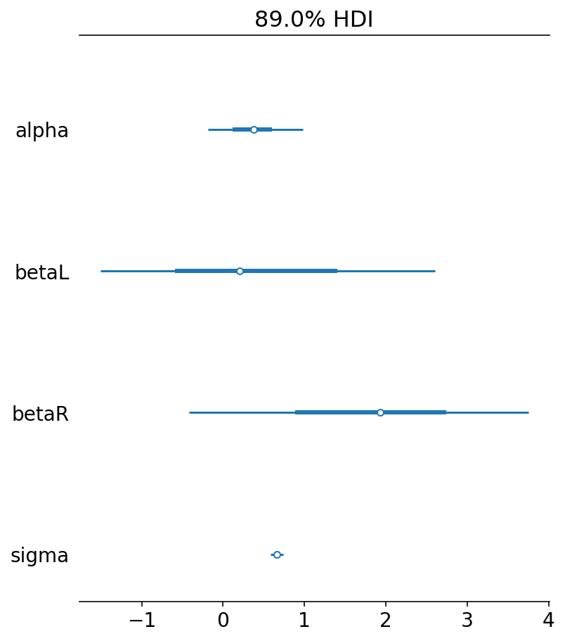
| betaL | 0.386 | 1.346 | -1.506 | 2.602 | 0.807 | 0.644 | 3.0 | 15.0 | 2.01 |
| betaR | 1.772 | 1.331 | -0.416 | 3.749 | 0.793 | 0.682 | 3.0 | 15.0 | 1.99 |
| sigma | 0.663 | 0.047 | 0.587 | 0.735 | 0.001 | 0.001 | 1322.0 | 1987.0 | 1.00 |
Notice betaL and betaR values. How can they be so different ? Afterall we know that the legs are more or less of same lenght so their effects should be both equal. This is confusing indeed !
az.plot_forest(trace_6_1, hdi_prob=0.89, combined=True)
array([<AxesSubplot:title={'center':'89.0% HDI'}>], dtype=object)
Code 6.5
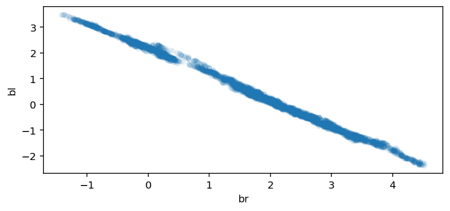
Looking at the bivariate posterior distribution for betaR & betaL.
Since both variables contain identical information, the posterior is a narrow ridge of negatively correlated values.
fig, ax = plt.subplots(1, 1, figsize=[7, 3])

plt.scatter(posterior_6_1["betaR"], posterior_6_1["betaL"], alpha=0.05, s=20)
ax.set_xlabel("br")
ax.set_ylabel("bl")
Text(0, 0.5, 'bl')
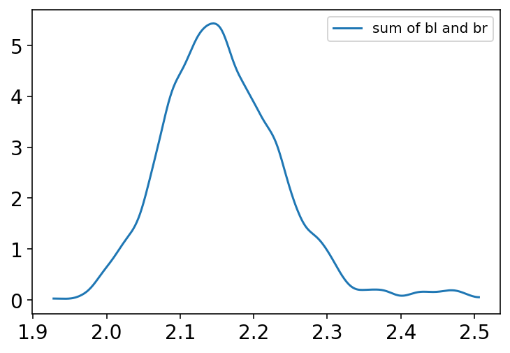
Code 6.6
Below plot shows that the posterior distribution of sum of the two parameters is centered on the proper association of either leg with height
sum_blbr = posterior_6_1["betaL"] + posterior_6_1["betaR"]
az.plot_kde(sum_blbr.numpy(), label="sum of bl and br");
Code 6.7
We will now do the regression using only one leg and the posterior mean will be approximately the same.
Building the model using only left leg.
def model_6_2(leg_left_data):
    def _generator():
        alpha = yield Root(
            tfd.Sample(tfd.Normal(loc=10.0, scale=100.0, name="alpha"), sample_shape=1)
        )
        betaL = yield Root(
            tfd.Sample(tfd.Normal(loc=2.0, scale=10.0, name="betaL"), sample_shape=1)
        )
        sigma = yield Root(
            tfd.Sample(tfd.Exponential(rate=1.0, name="sigma"), sample_shape=1)
        )

        mu = tf.squeeze(alpha[..., tf.newaxis] + betaL[..., tf.newaxis] * leg_left_data)

        scale = sigma[..., tf.newaxis]

        height = yield tfd.Independent(
            tfd.Normal(loc=mu, scale=scale, name="height"), reinterpreted_batch_ndims=1
        )

    return tfd.JointDistributionCoroutine(_generator, validate_args=False)


jdc_6_2 = model_6_2(tdf.leg_left)
NUM_CHAINS_FOR_6_2 = 2

# Note -
# I got somewhat ok looking results with this init values
init_state = [
    tf.ones([NUM_CHAINS_FOR_6_2]),
    tf.ones([NUM_CHAINS_FOR_6_2]),
    tf.ones([NUM_CHAINS_FOR_6_1]),
]

bijectors = [tfb.Identity(), tfb.Identity(), tfb.Exp()]

observed_data = (tdf.height,)

posterior_6_2, trace_6_2 = sample_posterior(
    jdc_6_2,
    observed_data=observed_data,
    num_chains=NUM_CHAINS_FOR_6_2,
    init_state=init_state,
    bijectors=bijectors,
    num_samples=4000,
    burnin=500,
    params=["alpha", "betaL", "sigma"],
)

az.summary(trace_6_2, hdi_prob=0.89)
| mean | sd | hdi_5.5% | hdi_94.5% | mcse_mean | mcse_sd | ess_bulk | ess_tail | r_hat | |
|---|---|---|---|---|---|---|---|---|---|
| alpha | 0.250 | 0.325 | -0.283 | 0.759 | 0.035 | 0.025 | 87.0 | 130.0 | 1.02 |
| betaL | 2.179 | 0.070 | 2.071 | 2.294 | 0.008 | 0.005 | 89.0 | 132.0 | 1.02 |
| sigma | 0.662 | 0.047 | 0.587 | 0.736 | 0.001 | 0.001 | 1496.0 | 2735.0 | 1.00 |
The value of betaL is now identical to sum of betaL & betaL (see the chart from Code 6.6) from previous models
6.1.2 Multicollinear milk
In real datasets, it may be difficult to identify the highly correlated predictors. This has the consequence of coming to a conclusion that none of the predictor is significant.
Here the primate milk dataset is used as another example for multicollinearity challenge.
Code 6.8
Loading the dataset and creating new standardized (centered) columns
d = RethinkingDataset.Milk.get_dataset()

d["K"] = d["kcal.per.g"].pipe(lambda x: (x - x.mean()) / x.std())
d["F"] = d["perc.fat"].pipe(lambda x: (x - x.mean()) / x.std())
d["L"] = d["perc.lactose"].pipe(lambda x: (x - x.mean()) / x.std())
tdf = dataframe_to_tensors("Milk", d, ["K", "F", "L"])
Code 6.9
We are building 2 models here.
KCal regressed on perc.fat
KCal regressed on perc.lactose
# KCal is regressed on perc.fat


def model_6_3(per_fat):
    def _generator():
        alpha = yield Root(
            tfd.Sample(tfd.Normal(loc=0.0, scale=0.2, name="alpha"), sample_shape=1)
        )
        betaF = yield Root(
            tfd.Sample(tfd.Normal(loc=0.0, scale=0.5, name="betaF"), sample_shape=1)
        )
        sigma = yield Root(
            tfd.Sample(tfd.Exponential(rate=1.0, name="sigma"), sample_shape=1)
        )

        mu = alpha[..., tf.newaxis] + betaF[..., tf.newaxis] * tf.transpose(
            per_fat[..., tf.newaxis]
        )
        scale = sigma[..., tf.newaxis]

        K = yield tfd.Independent(
            tfd.Normal(loc=mu, scale=scale, name="K"), reinterpreted_batch_ndims=1
        )

    return tfd.JointDistributionCoroutine(_generator, validate_args=False)


jdc_6_3 = model_6_3(tdf.F)
NUM_CHAINS_FOR_6_3 = 2

init_state = [
    tf.zeros([NUM_CHAINS_FOR_6_3]),
    tf.zeros([NUM_CHAINS_FOR_6_3]),
    tf.ones([NUM_CHAINS_FOR_6_3]),
]

bijectors = [tfb.Identity(), tfb.Identity(), tfb.Exp()]

posterior_6_3, trace_6_3 = sample_posterior(
    jdc_6_3,
    observed_data=(tdf.K,),
    init_state=init_state,
    bijectors=bijectors,
    params=["alpha", "betaF", "sigma"],
)
# KCal is regressed on perc.lactose


def model_6_4(per_lac):
    def _generator():
        alpha = yield Root(
            tfd.Sample(tfd.Normal(loc=0.0, scale=0.2, name="alpha"), sample_shape=1)
        )
        betaL = yield Root(
            tfd.Sample(tfd.Normal(loc=0.0, scale=0.5, name="betaL"), sample_shape=1)
        )
        sigma = yield Root(
            tfd.Sample(tfd.Exponential(rate=1.0, name="sigma"), sample_shape=1)
        )

        mu = alpha[..., tf.newaxis] + betaL[..., tf.newaxis] * tf.transpose(
            per_lac[..., tf.newaxis]
        )
        scale = sigma[..., tf.newaxis]

        K = yield tfd.Independent(
            tfd.Normal(loc=mu, scale=scale, name="K"), reinterpreted_batch_ndims=1
        )

    return tfd.JointDistributionCoroutine(_generator, validate_args=False)


jdc_6_4 = model_6_4(tdf.L)
NUM_CHAINS_FOR_6_4 = 2

init_state = [
    tf.zeros([NUM_CHAINS_FOR_6_4]),
    tf.zeros([NUM_CHAINS_FOR_6_4]),
    tf.ones([NUM_CHAINS_FOR_6_4]),
]

bijectors = [tfb.Identity(), tfb.Identity(), tfb.Exp()]

posterior_6_4, trace_6_4 = sample_posterior(
    jdc_6_4,
    observed_data=(tdf.K,),
    init_state=init_state,
    bijectors=bijectors,
    params=["alpha", "betaL", "sigma"],
)
az.summary(trace_6_3, hdi_prob=0.89)
| mean | sd | hdi_5.5% | hdi_94.5% | mcse_mean | mcse_sd | ess_bulk | ess_tail | r_hat | |
|---|---|---|---|---|---|---|---|---|---|
| alpha | 0.015 | 0.088 | -0.128 | 0.149 | 0.008 | 0.006 | 114.0 | 146.0 | 1.00 |
| betaF | 0.869 | 0.090 | 0.715 | 0.996 | 0.008 | 0.005 | 136.0 | 200.0 | 1.02 |
| sigma | 0.487 | 0.067 | 0.379 | 0.580 | 0.004 | 0.003 | 259.0 | 89.0 | 1.04 |
az.summary(trace_6_4, hdi_prob=0.89)
| mean | sd | hdi_5.5% | hdi_94.5% | mcse_mean | mcse_sd | ess_bulk | ess_tail | r_hat | |
|---|---|---|---|---|---|---|---|---|---|
| alpha | -0.001 | 0.077 | -0.110 | 0.136 | 0.007 | 0.005 | 115.0 | 199.0 | 1.02 |
| betaL | -0.898 | 0.080 | -1.023 | -0.777 | 0.005 | 0.004 | 264.0 | 411.0 | 1.01 |
| sigma | 0.414 | 0.059 | 0.319 | 0.494 | 0.002 | 0.001 | 1121.0 | 401.0 | 1.00 |
Posterior for betaF & betaL are mirror images of each other.
This seems to imply that both predictors have strong association with the outcome. Notice the sd of both the predictors; they are quite low.
In next section we will see what happens when we combine both of them in the regression model
Code 6.10
We build a model where we include both of the predictors (per_fat & per_lac)
def model_6_5(per_fat, per_lac):
    def _generator():
        alpha = yield Root(
            tfd.Sample(tfd.Normal(loc=0.0, scale=0.2, name="alpha"), sample_shape=1)
        )
        betaF = yield Root(
            tfd.Sample(tfd.Normal(loc=0.0, scale=0.5, name="betaF"), sample_shape=1)
        )
        betaL = yield Root(
            tfd.Sample(tfd.Normal(loc=0.0, scale=0.5, name="betaL"), sample_shape=1)
        )
        sigma = yield Root(
            tfd.Sample(tfd.Exponential(rate=1.0, name="sigma"), sample_shape=1)
        )

        mu = (
            alpha[..., tf.newaxis]
            + betaF[..., tf.newaxis] * tf.transpose(per_fat[..., tf.newaxis])
            + betaL[..., tf.newaxis] * tf.transpose(per_lac[..., tf.newaxis])
        )

        scale = sigma[..., tf.newaxis]

        K = yield tfd.Independent(
            tfd.Normal(loc=mu, scale=scale, name="K"), reinterpreted_batch_ndims=1
        )

    return tfd.JointDistributionCoroutine(_generator, validate_args=False)


jdc_6_5 = model_6_5(tdf.F, tdf.L)
NUM_CHAINS_FOR_6_5 = 2

init_state = [
    tf.zeros([NUM_CHAINS_FOR_6_5]),
    tf.zeros([NUM_CHAINS_FOR_6_5]),
    tf.zeros([NUM_CHAINS_FOR_6_5]),
    tf.ones([NUM_CHAINS_FOR_6_5]),
]

bijectors = [tfb.Identity(), tfb.Identity(), tfb.Identity(), tfb.Exp()]

posterior_6_5, trace_6_5 = sample_posterior(
    jdc_6_5,
    observed_data=(tdf.K,),
    num_chains=NUM_CHAINS_FOR_6_5,
    init_state=init_state,
    bijectors=bijectors,
    params=["alpha", "betaF", "betaL", "sigma"],
)

az.summary(trace_6_5, hdi_prob=0.89)
WARNING:tensorflow:5 out of the last 5 calls to <function run_hmc_chain at 0x7f6409dec710> triggered tf.function retracing. Tracing is expensive and the excessive number of tracings could be due to (1) creating @tf.function repeatedly in a loop, (2) passing tensors with different shapes, (3) passing Python objects instead of tensors. For (1), please define your @tf.function outside of the loop. For (2), @tf.function has experimental_relax_shapes=True option that relaxes argument shapes that can avoid unnecessary retracing. For (3), please refer to https://www.tensorflow.org/guide/function#controlling_retracing and https://www.tensorflow.org/api_docs/python/tf/function for more details.
| mean | sd | hdi_5.5% | hdi_94.5% | mcse_mean | mcse_sd | ess_bulk | ess_tail | r_hat | |
|---|---|---|---|---|---|---|---|---|---|
| alpha | -0.006 | 0.068 | -0.112 | 0.100 | 0.004 | 0.003 | 250.0 | 457.0 | 1.01 |
| betaF | 0.260 | 0.197 | -0.022 | 0.564 | 0.015 | 0.010 | 170.0 | 200.0 | 1.01 |
| betaL | -0.659 | 0.204 | -0.964 | -0.347 | 0.016 | 0.012 | 149.0 | 129.0 | 1.01 |
| sigma | 0.413 | 0.063 | 0.321 | 0.511 | 0.003 | 0.002 | 361.0 | 196.0 | 1.02 |
Notice how the standard deviations of the posterior for betaF & betaL has jumped up significantly.
per_fat & per_lac both contain much of the same information and can be substitued for each other. Therefore, the model has not choice but to describe a long ridge of combination of betaF & betaL that are equally plaussible.
Code 6.11
We plot again like in the legs example to visualize the relationship
az.plot_pair(d[["kcal.per.g", "perc.fat", "perc.lactose"]].to_dict("list"));
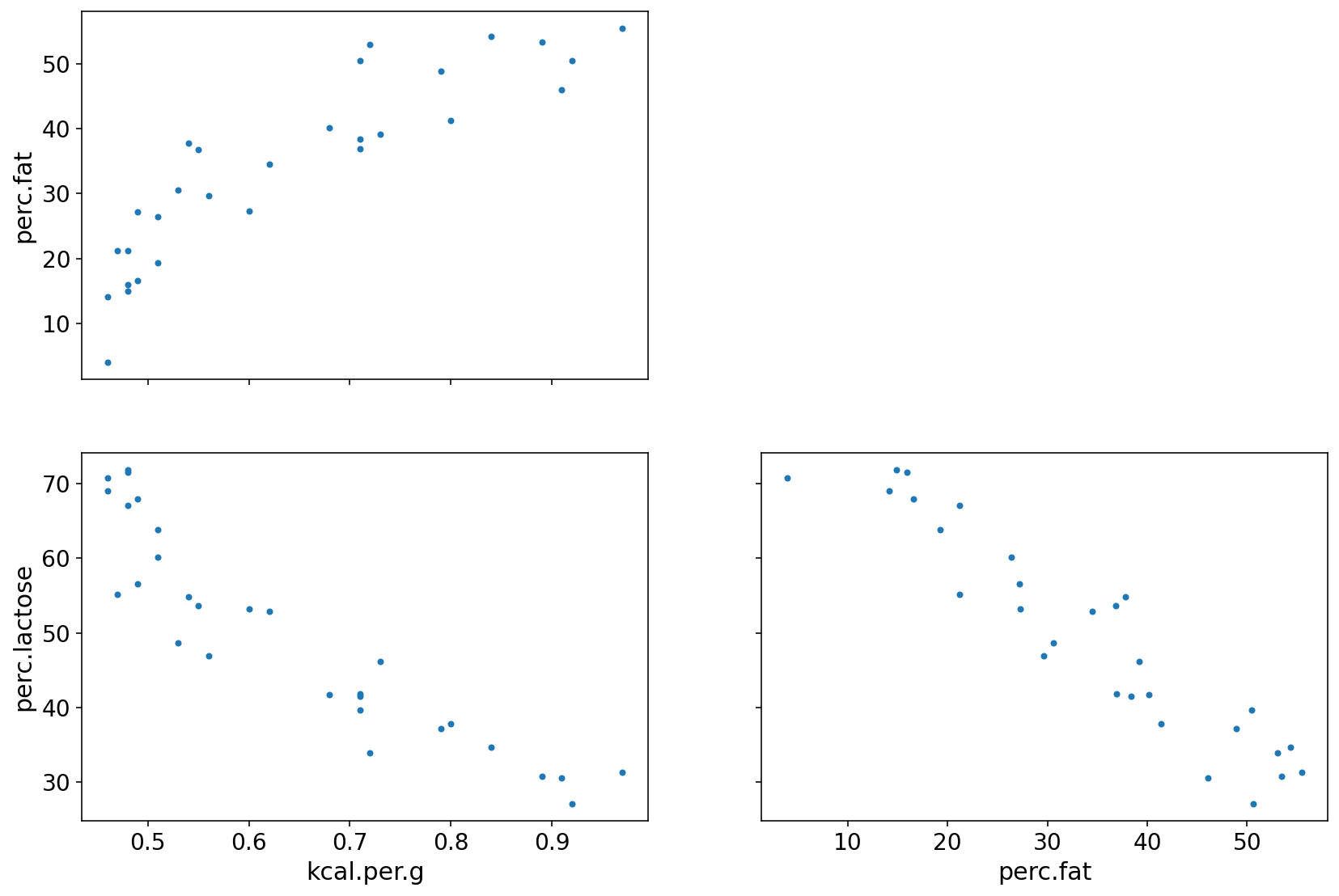
perc.fat is positively related to outcome
perc.lac is negatively related to outcome
perc.fat & perc.lac are negatively coorelated to each other
Either of them helps in predicting KCal but neither helps much once we already know the other.
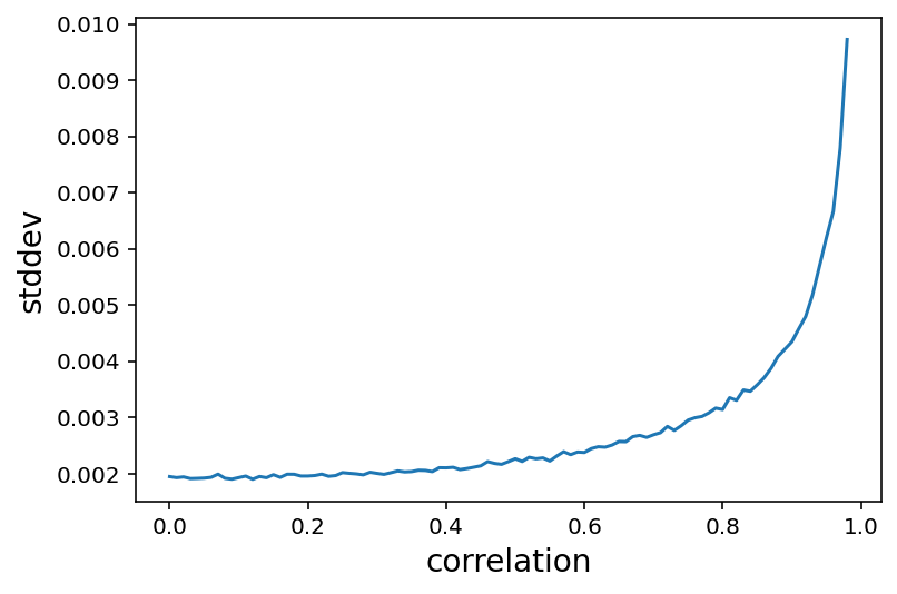
Overthinking : Simulating collinearity
Simulating collinearity using Milk dataset
Code 6.12
d = RethinkingDataset.Milk.get_dataset()


def simcoll(r=0.9):

    mean = r * d["perc.fat"].values
    sd = np.sqrt((1 - r ** 2) * np.var(d["perc.fat"].values))

    x = tfd.Normal(loc=mean, scale=sd).sample()

    X = np.column_stack((d["perc.fat"], x))
    m = linear_model.OLS(d["kcal.per.g"], X).fit()
    cov = m.cov_params()
    return (np.diag(cov)[1]) ** 0.5


def repsimcoll(r=0.9, N=100):
    stddev = [simcoll(r) for _ in range(N)]
    return np.mean(stddev)


lista = []
for i in np.arange(start=0, stop=0.99, step=0.01):
    lista.append(repsimcoll(r=i, N=100))

plt.plot(np.arange(start=0, stop=0.99, step=0.01), lista)
plt.xlabel("correlation", fontsize=14)
plt.ylabel("stddev", fontsize=14);
6.2 Post-treatment bias
Omitted Variable bias - Problems that arise because of not including predictior variables
Post-treatment bias - Problems that arise becuase of including improper predictor variables
Code 6.13
Simulate data to see what goes wrong when we include a post-treatment variable
_SEED = 71

# Note - even after providing SeedStream and generated seeds
# it still does not respect it
def simulate():
    seed = tfp.util.SeedStream(_SEED, salt="sim_heights")

    # number of plants
    N = 100

    # simulate initial heights
    h0 = tfd.Normal(loc=10.0, scale=2.0).sample(N, seed=seed())

    # assign treatments and simulate fungus and growth
    treatment = tf.repeat([0.0, 1.0], repeats=N // 2)

    fungus = tfd.Binomial(total_count=1.0, probs=(0.5 - treatment * 0.4)).sample(
        seed=seed()
    )

    h1 = h0 + tfd.Normal(loc=5.0 - 3.0 * fungus, scale=1.0).sample(seed=seed())

    # compose a clean data frame
    d = {"h0": h0, "h1": h1, "treatment": treatment, "fungus": fungus}

    return d


d_dict = simulate()

az.summary(d_dict, kind="stats", hdi_prob=0.89)
| mean | sd | hdi_5.5% | hdi_94.5% | |
|---|---|---|---|---|
| h0 | 9.894 | 2.143 | 6.421 | 12.93 |
| h1 | 13.609 | 2.696 | 8.782 | 17.34 |
| treatment | 0.500 | 0.503 | 0.000 | 1.00 |
| fungus | 0.350 | 0.479 | 0.000 | 1.00 |
d = pd.DataFrame.from_dict(d_dict)
tdf = dataframe_to_tensors("SimulatedTreatment", d, ["h0", "h1", "treatment", "fungus"])
6.2.1 A prior is born
We will use a prior (see Code 6.14) that expects anything from 40% shrinkage up to 50% growth
Code 6.14
sim_p = tfd.LogNormal(loc=0.0, scale=0.25).sample((int(1e4),))
az.summary({"sim_p": sim_p}, kind="stats", hdi_prob=0.89)
| mean | sd | hdi_5.5% | hdi_94.5% | |
|---|---|---|---|---|
| sim_p | 1.031 | 0.261 | 0.648 | 1.438 |
Code 6.15
In this model only height (h0) as the predictor is included
def model_6_6(h0):
    def _generator():
        p = yield Root(
            tfd.Sample(tfd.LogNormal(loc=0.0, scale=0.25, name="p"), sample_shape=1)
        )
        sigma = yield Root(
            tfd.Sample(tfd.Exponential(rate=1.0, name="sigma"), sample_shape=1)
        )

        mu = tf.squeeze(h0[tf.newaxis, ...] * p[..., tf.newaxis])
        scale = sigma[..., tf.newaxis]

        h1 = yield tfd.Independent(
            tfd.Normal(loc=mu, scale=scale, name="h1"), reinterpreted_batch_ndims=1
        )

    return tfd.JointDistributionCoroutine(_generator, validate_args=False)


jdc_6_6 = model_6_6(tdf.h0)
NUM_CHAINS_FOR_6_6 = 2

init_state = [tf.ones([NUM_CHAINS_FOR_6_6]), tf.ones([NUM_CHAINS_FOR_6_6])]

bijectors = [tfb.Exp(), tfb.Exp()]

posterior_6_6, trace_6_6 = sample_posterior(
    jdc_6_6,
    observed_data=(tdf.h1,),
    num_chains=NUM_CHAINS_FOR_6_6,
    init_state=init_state,
    bijectors=bijectors,
    num_samples=2000,
    burnin=1000,
    params=["p", "sigma"],
)

az.summary(trace_6_6, hdi_prob=0.89)
WARNING:tensorflow:6 out of the last 6 calls to <function run_hmc_chain at 0x7f6409dec710> triggered tf.function retracing. Tracing is expensive and the excessive number of tracings could be due to (1) creating @tf.function repeatedly in a loop, (2) passing tensors with different shapes, (3) passing Python objects instead of tensors. For (1), please define your @tf.function outside of the loop. For (2), @tf.function has experimental_relax_shapes=True option that relaxes argument shapes that can avoid unnecessary retracing. For (3), please refer to https://www.tensorflow.org/guide/function#controlling_retracing and https://www.tensorflow.org/api_docs/python/tf/function for more details.
| mean | sd | hdi_5.5% | hdi_94.5% | mcse_mean | mcse_sd | ess_bulk | ess_tail | r_hat | |
|---|---|---|---|---|---|---|---|---|---|
| p | 1.357 | 0.020 | 1.324 | 1.387 | 0.000 | 0.000 | 1981.0 | 1291.0 | 1.00 |
| sigma | 1.907 | 0.135 | 1.691 | 2.113 | 0.004 | 0.003 | 1040.0 | 1010.0 | 1.01 |
The result shows that with height as the only predictor variable in the model there is about 40% growth on average.
Code 6.16
In this model we include treatment & fungus variables as well
def model_6_7(h0, treatment, fungus):
    def _generator():
        a = yield Root(
            tfd.Sample(tfd.LogNormal(loc=0.0, scale=0.2, name="a"), sample_shape=1)
        )
        bt = yield Root(
            tfd.Sample(tfd.Normal(loc=0.0, scale=0.5, name="bt"), sample_shape=1)
        )
        bf = yield Root(
            tfd.Sample(tfd.Normal(loc=0.0, scale=0.5, name="bf"), sample_shape=1)
        )
        sigma = yield Root(
            tfd.Sample(tfd.Exponential(rate=1.0, name="sigma"), sample_shape=1)
        )

        p = (
            a[..., tf.newaxis]
            + bt[..., tf.newaxis] * treatment
            + bf[..., tf.newaxis] * fungus
        )

        mu = h0 * p
        scale = sigma[..., tf.newaxis]

        h1 = yield tfd.Independent(
            tfd.Normal(loc=mu, scale=scale, name="h1"), reinterpreted_batch_ndims=1
        )

    return tfd.JointDistributionCoroutine(_generator, validate_args=False)


jdc_6_7 = model_6_7(tdf.h0, tdf.treatment, tdf.fungus)
NUM_CHAINS_FOR_6_7 = 2

init_state = [
    tf.ones([NUM_CHAINS_FOR_6_7]),
    tf.zeros([NUM_CHAINS_FOR_6_7]),
    tf.zeros([NUM_CHAINS_FOR_6_7]),
    tf.ones([NUM_CHAINS_FOR_6_7]),
]

bijectors = [tfb.Exp(), tfb.Identity(), tfb.Identity(), tfb.Exp()]

posterior_6_7, trace_6_7 = sample_posterior(
    jdc_6_7,
    observed_data=(tdf.h1,),
    num_chains=NUM_CHAINS_FOR_6_7,
    init_state=init_state,
    bijectors=bijectors,
    num_samples=2000,
    burnin=1000,
    params=["a", "bt", "bf", "sigma"],
)

az.summary(trace_6_7, hdi_prob=0.89)
| mean | sd | hdi_5.5% | hdi_94.5% | mcse_mean | mcse_sd | ess_bulk | ess_tail | r_hat | |
|---|---|---|---|---|---|---|---|---|---|
| a | 1.455 | 0.029 | 1.409 | 1.501 | 0.001 | 0.001 | 1039.0 | 1136.0 | 1.00 |
| bt | -0.011 | 0.034 | -0.070 | 0.037 | 0.001 | 0.001 | 1254.0 | 1324.0 | 1.00 |
| bf | -0.277 | 0.036 | -0.328 | -0.214 | 0.001 | 0.001 | 1213.0 | 1114.0 | 1.00 |
| sigma | 1.388 | 0.099 | 1.240 | 1.551 | 0.005 | 0.003 | 410.0 | 657.0 | 1.01 |
Note that a is same as p in the previous model i.e. about 40% growth on average
Marginal posterior for bt (effect of treatment) is about 0 with a tight interval. This implies treatment is not associated with the growth.
Fungus (bf) seems to actually hurt the growth.
Clearly this does not makes us happy because we know that the treatment does matter. Next section tries to find the answers.
6.2.2 Blocked by consequence
Fungus is a consequence of treatment i.e. fungus is a post-treatment variable.
When we include Fungus variable, the model tries to find whether a plat developed fungus or not. However, what we really want to understand is the impact of treatment on growth.
This can be done by omitting the post-treatment variable fungus
Code 6.17
In this model, fungus predictor is not included
def model_6_8(h0, treatment):
    def _generator():
        a = yield Root(
            tfd.Sample(tfd.LogNormal(loc=0.0, scale=0.2, name="a"), sample_shape=1)
        )
        bt = yield Root(
            tfd.Sample(tfd.Normal(loc=0.0, scale=0.5, name="bt"), sample_shape=1)
        )
        sigma = yield Root(
            tfd.Sample(tfd.Exponential(rate=1.0, name="sigma"), sample_shape=1)
        )

        p = a[..., tf.newaxis] + bt[..., tf.newaxis] * treatment

        mu = h0 * p
        scale = sigma[..., tf.newaxis]

        h1 = yield tfd.Independent(
            tfd.Normal(loc=mu, scale=scale, name="h1"), reinterpreted_batch_ndims=1
        )

    return tfd.JointDistributionCoroutine(_generator, validate_args=False)


jdc_6_8 = model_6_8(tdf.h0, tdf.treatment)
NUM_CHAINS_FOR_6_8 = 2

init_state = [
    tf.ones([NUM_CHAINS_FOR_6_8]),
    tf.zeros([NUM_CHAINS_FOR_6_8]),
    tf.ones([NUM_CHAINS_FOR_6_8]),
]

bijectors = [tfb.Exp(), tfb.Identity(), tfb.Exp()]

posterior_6_8, trace_6_8 = sample_posterior(
    jdc_6_8,
    observed_data=(tdf.h1,),
    num_chains=NUM_CHAINS_FOR_6_8,
    init_state=init_state,
    bijectors=bijectors,
    num_samples=2000,
    burnin=1000,
    params=["a", "bt", "sigma"],
)

az.summary(trace_6_8, hdi_prob=0.89)
| mean | sd | hdi_5.5% | hdi_94.5% | mcse_mean | mcse_sd | ess_bulk | ess_tail | r_hat | |
|---|---|---|---|---|---|---|---|---|---|
| a | 1.287 | 0.025 | 1.247 | 1.326 | 0.001 | 0.000 | 2245.0 | 1777.0 | 1.0 |
| bt | 0.134 | 0.036 | 0.081 | 0.194 | 0.001 | 0.000 | 3878.0 | 1516.0 | 1.0 |
| sigma | 1.798 | 0.128 | 1.587 | 1.990 | 0.004 | 0.003 | 1086.0 | 1481.0 | 1.0 |
We can now see that bt (effect of treatment) has a positive impact on the model.
6.2.3 Fungus and d-separation
Above we built models by including and excluding various potential predictors. However, it helps to represent these relations graphically with the help of DAG.
Code 6.18
Here we are using causalgraphicalmodel package
plant_dag = CausalGraphicalModel(
    nodes=["H0", "H1", "F", "T"], edges=[("H0", "H1"), ("F", "H1"), ("T", "F")]
)
pgm = daft.PGM()
coordinates = {"H0": (0, 0), "T": (4, 0), "F": (3, 0), "H1": (2, 0)}
for node in plant_dag.dag.nodes:
    pgm.add_node(node, node, *coordinates[node])
for edge in plant_dag.dag.edges:
    pgm.add_edge(*edge)
pgm.render()
plt.gca().invert_yaxis()
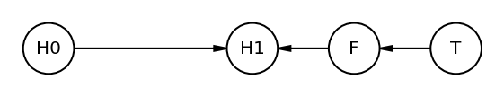
The graph clearly shows how treatment’s (T) impact on height (H1) is blocked by fungus (F)
Another way to say above is - If we condition on F it induces D-SEPARATION. The “d” stands for directional
H1 is conditionally independent of T if we include F (the blocker)
Code 6.19
all_independencies = plant_dag.get_all_independence_relationships()
for s in all_independencies:
    if all(
        t[0] != s[0] or t[1] != s[1] or not t[2].issubset(s[2])
        for t in all_independencies
        if t != s
    ):
        print(s)
('F', 'H0', set())
('T', 'H1', {'F'})
('T', 'H0', set())
Here is how we want to read the above result -
H0 is conditionally independent on T (note the empty set). In other words, original height H0 should not be associated with T
H0 is conditionally independent on F (note the empty set). In other words, original height H0 should not be associated with F
H1 is conditionally independent on T if we include F
Code 6.20
A synthetic data generation to modifiy the plant growth simulation so that fungus has no influence on growth, but moisture M influences both H1 and F
_SEED = 71

# Note - even after providing SeedStream and generated seeds
# it still does not respect it
def simulate():
    seed = tfp.util.SeedStream(_SEED, salt="sim_heights")

    # number of plants
    N = 1000

    # simulate initial heights
    h0 = tfd.Normal(loc=10.0, scale=2.0).sample(N, seed=seed())

    # assign treatments and simulate fungus and growth
    treatment = tf.repeat([0.0, 1.0], repeats=N // 2)

    M = tf.cast(tfd.Bernoulli(probs=0.5).sample(N, seed=seed()), dtype=tf.float32)

    fungus = tfd.Binomial(
        total_count=1.0, probs=(0.5 - treatment * 0.4 + M * 0.4)
    ).sample(seed=seed())

    h1 = h0 + tfd.Normal(loc=5.0 + 3.0 * M, scale=1.0).sample(seed=seed())

    # compose a clean data frame
    d = {"h0": h0, "h1": h1, "treatment": treatment, "fungus": fungus}

    return d


d = simulate()

az.summary(d, kind="stats", hdi_prob=0.89)
| mean | sd | hdi_5.5% | hdi_94.5% | |
|---|---|---|---|---|
| h0 | 9.994 | 2.06 | 6.494 | 12.935 |
| h1 | 16.544 | 2.80 | 12.268 | 20.809 |
| treatment | 0.500 | 0.50 | 0.000 | 1.000 |
| fungus | 0.491 | 0.50 | 0.000 | 1.000 |
6.3 Collider bias
6.3.1 Collider of false sorrow
Question we consider in this section is how aging influences happiness ?
We also know that happiness (H) & age (A) both cause marriage (M). This makes marriage (M) a collider
H —-> M <—– A
Code 6.21
Simulating (synthetic data generation) happiness and its relationship with age & marriage
Each year, 20 people are born with uniformly distributed happiness values
Each year, each person ages one year. Happiness does not change.
At age 18, individuals can be married. The odds of marriage each year are proportional to an individual’s happiness
Once married, an individual remains married
After age 65, individuals leave the sample. (They move to Spain)
# Port of R code from here https://github.com/rmcelreath/rethinking/blob/master/R/sim_happiness.R
def sim_happiness(seed=1977, N_years=1000, max_age=65, N_births=20, aom=18):
    # age existing individuals & newborns
    A = np.repeat(np.arange(1, N_years + 1), N_births)
    # sim happiness trait - never changes
    H = np.repeat(np.linspace(-2, 2, N_births)[None, :], N_years, 0).reshape(-1)
    # not yet married
    M = np.zeros(N_years * N_births, dtype=np.uint8)

    def update_M(i, M):
        # for each person over 17, chance get married
        married = tfd.Bernoulli(logits=(H - 4.0)).sample(seed=seed + i).numpy()
        return np.where((A >= i) & (M == 0.0), married, M)

    def fori_loop(lower, upper, body_fun, init_val):
        val = init_val
        for i in range(lower, upper):
            val = body_fun(i, val)
        return val

    M = fori_loop(aom, max_age + 1, update_M, M)

    # mortality
    deaths = A > max_age
    A = A[~deaths]
    H = H[~deaths]
    M = M[~deaths]

    d = pd.DataFrame({"age": A, "married": M, "happiness": H})
    return d


d = sim_happiness(seed=1977, N_years=1000)
d.describe()
| age | married | happiness | |
|---|---|---|---|
| count | 1300.000000 | 1300.000000 | 1.300000e+03 |
| mean | 33.000000 | 0.292308 | -8.335213e-17 |
| std | 18.768883 | 0.454998 | 1.214421e+00 |
| min | 1.000000 | 0.000000 | -2.000000e+00 |
| 25% | 17.000000 | 0.000000 | -1.000000e+00 |
| 50% | 33.000000 | 0.000000 | -1.110223e-16 |
| 75% | 49.000000 | 1.000000 | 1.000000e+00 |
| max | 65.000000 | 1.000000 | 2.000000e+00 |
Code 6.22
Rescaling age so that the range from 18 to 65 is one unit
We are adding a new column called “A” that ranges from 0 to 1 where 0 is age 18 and 1 is age 65
Happiness is on an arbitary scale from -2 to +2
d2 = d[d.age > 17].copy()  # only adults
d2["A"] = (d2.age - 18) / (65 - 18)
Code 6.23
Here we are doing multiple regression. The linear model is
\(\mu_i\) = \(\alpha_{MID[i]}\) + \(\beta_A\) * \(A_i\)
d2["mid"] = d2.married

tdf = dataframe_to_tensors(
    "SimulatedHappiness",
    d2,
    {"mid": tf.int32, "A": tf.float32, "happiness": tf.float32},
)


def model_6_9(mid, A):
    def _generator():
        a = yield Root(
            tfd.Sample(tfd.Normal(loc=0.0, scale=1.0, name="a"), sample_shape=2)
        )
        bA = yield Root(
            tfd.Sample(tfd.Normal(loc=0.0, scale=2.0, name="bA"), sample_shape=1)
        )
        sigma = yield Root(
            tfd.Sample(tfd.Exponential(rate=1.0, name="sigma"), sample_shape=1)
        )

        mu = tf.squeeze(tf.gather(a, mid, axis=-1)) + bA[..., tf.newaxis] * A
        scale = sigma[..., tf.newaxis]

        h = yield tfd.Independent(
            tfd.Normal(loc=mu, scale=scale, name="h"), reinterpreted_batch_ndims=1
        )

    return tfd.JointDistributionCoroutine(_generator, validate_args=False)


jdc_6_9 = model_6_9(mid=tdf.mid, A=tdf.A)
NUM_CHAINS_FOR_6_9 = 2

init_state = [
    tf.ones([NUM_CHAINS_FOR_6_9, 2]),
    tf.zeros([NUM_CHAINS_FOR_6_9]),
    tf.ones([NUM_CHAINS_FOR_6_9]),
]

bijectors = [tfb.Identity(), tfb.Identity(), tfb.Exp()]

observed_value = (tdf.happiness,)

posterior_6_9, trace_6_9 = sample_posterior(
    jdc_6_9,
    observed_data=observed_value,
    num_chains=NUM_CHAINS_FOR_6_9,
    init_state=init_state,
    bijectors=bijectors,
    num_samples=2000,
    burnin=1000,
    params=["a", "bA", "sigma"],
)

az.summary(trace_6_9, hdi_prob=0.89)
| mean | sd | hdi_5.5% | hdi_94.5% | mcse_mean | mcse_sd | ess_bulk | ess_tail | r_hat | |
|---|---|---|---|---|---|---|---|---|---|
| a[0] | -0.192 | 0.063 | -0.296 | -0.096 | 0.002 | 0.001 | 1067.0 | 1691.0 | 1.0 |
| a[1] | 1.333 | 0.087 | 1.207 | 1.486 | 0.003 | 0.002 | 892.0 | 1366.0 | 1.0 |
| bA | -0.827 | 0.114 | -1.019 | -0.654 | 0.004 | 0.003 | 760.0 | 983.0 | 1.0 |
| sigma | 0.990 | 0.023 | 0.954 | 1.023 | 0.001 | 0.000 | 1146.0 | 1893.0 | 1.0 |
The model here is quite sure that age is negatively associated with happiness.
Code 6.24
What would happen if omit the marriage status ?
Note - \(a\) is not any more a vector; just a plain intercept
def model_6_10(A):
    def _generator():
        a = yield Root(
            tfd.Sample(tfd.Normal(loc=0.0, scale=1.0, name="a"), sample_shape=1)
        )
        bA = yield Root(
            tfd.Sample(tfd.Normal(loc=0.0, scale=2.0, name="bA"), sample_shape=1)
        )
        sigma = yield Root(
            tfd.Sample(tfd.Exponential(rate=1.0, name="sigma"), sample_shape=1)
        )

        mu = a[..., tf.newaxis] + bA[..., tf.newaxis] * A
        scale = sigma[..., tf.newaxis]

        h = yield tfd.Independent(
            tfd.Normal(loc=mu, scale=scale, name="h"), reinterpreted_batch_ndims=1
        )

    return tfd.JointDistributionCoroutine(_generator, validate_args=False)


jdc_6_10 = model_6_10(A=tdf.A)
NUM_CHAINS_FOR_6_10 = 2

init_state = [
    tf.ones([NUM_CHAINS_FOR_6_10]),
    tf.zeros([NUM_CHAINS_FOR_6_10]),
    tf.ones([NUM_CHAINS_FOR_6_10]),
]

bijectors = [tfb.Identity(), tfb.Identity(), tfb.Exp()]

observed_value = (tdf.happiness,)

posterior_6_10, trace_6_10 = sample_posterior(
    jdc_6_10,
    observed_data=observed_value,
    num_chains=NUM_CHAINS_FOR_6_10,
    init_state=init_state,
    bijectors=bijectors,
    num_samples=2000,
    burnin=1000,
    params=["a", "bA", "sigma"],
)

az.summary(trace_6_10, hdi_prob=0.89)
| mean | sd | hdi_5.5% | hdi_94.5% | mcse_mean | mcse_sd | ess_bulk | ess_tail | r_hat | |
|---|---|---|---|---|---|---|---|---|---|
| a | 0.002 | 0.077 | -0.122 | 0.122 | 0.002 | 0.002 | 1017.0 | 1369.0 | 1.0 |
| bA | -0.005 | 0.133 | -0.216 | 0.196 | 0.004 | 0.003 | 927.0 | 1288.0 | 1.0 |
| sigma | 1.216 | 0.028 | 1.172 | 1.262 | 0.000 | 0.000 | 4132.0 | 1532.0 | 1.0 |
The value is \(a\) is close to zero. This implies that the model finds no association between age and happiness.
The pattern above is exactly what we should expect when condition on a collider. Here the collider is marriage status. It is a common consequence of age and happiness and therefore if we condition on it we are bound to induce a spurious association between the two causes
6.3.2 The hanted DAG
Collider may not be easily avoidable because they may be unmesasured causes. “Unmeasured” => Our DAG is haunted
Code 6.25
Here we will simulate another dataset using which we will try to infer the direct influene of both parents (P) and grandparents (G) on the educational achievement of childern (C)
It should be obvious that G -> P, P->C and G->C
N = 200  # number of grandparent-parent-child triads
b_GP = 1.0  # direct effect of G on P
b_GC = 0.0  # direct effect of G on C
b_PC = 1.0  # direct effect of P on C
b_U = 2.0  # direct effect of U on P and C
Code 6.26
Here is our “functional” (relationship) modeling
P is some function of G & U
C is some function of G, P & U
G & U are not functions of any other known variables
def grand_parent_sim():
    seed = tfp.util.SeedStream(1, salt="sim_grand_parent")
    U = 2 * tfd.Bernoulli(probs=0.5).sample(seed=seed(), sample_shape=N) - 1
    G = tfd.Normal(loc=0.0, scale=1.0).sample(seed=seed(), sample_shape=N)
    temp = b_GP * G + b_U * tf.cast(U, dtype=tf.float32)
    P = tfd.Normal(loc=temp, scale=1.0).sample(seed=seed())
    temp2 = b_PC * P + b_GC * G + b_U * tf.cast(U, dtype=tf.float32)
    C = tfd.Normal(loc=temp2, scale=1.0).sample(seed=seed())

    d = pd.DataFrame({"C": C.numpy(), "P": P.numpy(), "G": G.numpy(), "U": U.numpy()})

    return d


d = grand_parent_sim()

d
| C | P | G | U | |
|---|---|---|---|---|
| 0 | 3.512862 | 1.650976 | -1.042326 | 1 |
| 1 | -4.590997 | -1.555232 | 0.232263 | -1 |
| 2 | 4.886199 | 3.082321 | 1.986989 | 1 |
| 3 | 1.636396 | 1.243976 | -1.034003 | 1 |
| 4 | -8.797684 | -5.349887 | -3.269576 | -1 |
| ... | ... | ... | ... | ... |
| 195 | 3.745021 | 0.391891 | 0.254253 | 1 |
| 196 | -4.513893 | -2.212740 | -1.100699 | -1 |
| 197 | -3.206512 | -0.455612 | 0.602985 | -1 |
| 198 | 1.082468 | -0.115803 | 0.106212 | 1 |
| 199 | -2.545109 | 0.838045 | 2.178708 | -1 |
200 rows × 4 columns
tdf = dataframe_to_tensors("SimulatedEducation", d, ["P", "G", "C", "U"])
Code 6.27
Simple regression of C on P & G
def model_6_11(P, G):
    def _generator():
        a = yield Root(
            tfd.Sample(tfd.Normal(loc=0.0, scale=1.0, name="a"), sample_shape=1)
        )
        b_PC = yield Root(
            tfd.Sample(tfd.Normal(loc=0.0, scale=1.0, name="b_PC"), sample_shape=1)
        )
        b_GC = yield Root(
            tfd.Sample(tfd.Normal(loc=0.0, scale=1.0, name="b_GC"), sample_shape=1)
        )
        sigma = yield Root(
            tfd.Sample(tfd.Exponential(rate=1.0, name="sigma"), sample_shape=1)
        )

        mu = a[..., tf.newaxis] + b_PC[..., tf.newaxis] * P + b_GC[..., tf.newaxis] * G
        scale = sigma[..., tf.newaxis]

        h = yield tfd.Independent(
            tfd.Normal(loc=mu, scale=scale, name="h"), reinterpreted_batch_ndims=1
        )

    return tfd.JointDistributionCoroutine(_generator, validate_args=False)


jdc_6_11 = model_6_11(P=tdf.P, G=tdf.G)
NUM_CHAINS_FOR_6_11 = 2

init_state = [
    tf.zeros([NUM_CHAINS_FOR_6_11]),
    tf.ones([NUM_CHAINS_FOR_6_11]),
    tf.ones([NUM_CHAINS_FOR_6_11]),
    tf.ones([NUM_CHAINS_FOR_6_11]),
]

bijectors = [tfb.Identity(), tfb.Identity(), tfb.Identity(), tfb.Exp()]

observed_value = (tdf.C,)

posterior_6_11, trace_6_11 = sample_posterior(
    jdc_6_11,
    observed_data=observed_value,
    num_chains=NUM_CHAINS_FOR_6_11,
    init_state=init_state,
    bijectors=bijectors,
    num_samples=4000,
    burnin=1000,
    params=["a", "bPC", "bGC", "sigma"],
)

az.summary(trace_6_11, hdi_prob=0.89)
| mean | sd | hdi_5.5% | hdi_94.5% | mcse_mean | mcse_sd | ess_bulk | ess_tail | r_hat | |
|---|---|---|---|---|---|---|---|---|---|
| a | 0.056 | 0.096 | -0.084 | 0.224 | 0.001 | 0.002 | 8955.0 | 1666.0 | 1.0 |
| bPC | 1.818 | 0.045 | 1.746 | 1.889 | 0.001 | 0.000 | 4429.0 | 3198.0 | 1.0 |
| bGC | -0.897 | 0.101 | -1.065 | -0.750 | 0.001 | 0.001 | 7395.0 | 1906.0 | 1.0 |
| sigma | 1.382 | 0.072 | 1.263 | 1.491 | 0.003 | 0.002 | 791.0 | 1431.0 | 1.0 |
The inferred effect of parents looks too big, almost twice as large as it should be i.e. 1 vs 1.8
Some correlation between P & C is due to U and that’s a simple confound.
Interestingly model is confident (bGC) that the direct effect of grandparents is to hurt their grandkids
Code 6.28
Regression that conditions on U as well
def model_6_12(P, G, U):
    def _generator():
        a = yield Root(
            tfd.Sample(tfd.Normal(loc=0.0, scale=1.0, name="a"), sample_shape=1)
        )
        b_PC = yield Root(
            tfd.Sample(tfd.Normal(loc=0.0, scale=1.0, name="b_PC"), sample_shape=1)
        )
        b_GC = yield Root(
            tfd.Sample(tfd.Normal(loc=0.0, scale=1.0, name="b_GC"), sample_shape=1)
        )
        b_U = yield Root(
            tfd.Sample(tfd.Normal(loc=0.0, scale=1.0, name="b_U"), sample_shape=1)
        )
        sigma = yield Root(
            tfd.Sample(tfd.Exponential(rate=1.0, name="sigma"), sample_shape=1)
        )

        mu = (
            a[..., tf.newaxis]
            + b_PC[..., tf.newaxis] * P
            + b_GC[..., tf.newaxis] * G
            + b_U[..., tf.newaxis] * U
        )

        scale = sigma[..., tf.newaxis]

        h = yield tfd.Independent(
            tfd.Normal(loc=mu, scale=scale, name="h"), reinterpreted_batch_ndims=1
        )

    return tfd.JointDistributionCoroutine(_generator, validate_args=False)


jdc_6_12 = model_6_12(P=tdf.P, G=tdf.G, U=tdf.U)
NUM_CHAINS_FOR_6_12 = 2

init_state = [
    tf.zeros([NUM_CHAINS_FOR_6_12]),
    tf.zeros([NUM_CHAINS_FOR_6_12]),
    tf.zeros([NUM_CHAINS_FOR_6_12]),
    tf.ones([NUM_CHAINS_FOR_6_12]),  # <-- note 1 instead of zero here. Necessary !!
    tf.ones([NUM_CHAINS_FOR_6_12]),
]

bijectors = [tfb.Identity(), tfb.Identity(), tfb.Identity(), tfb.Identity(), tfb.Exp()]

observed_value = (tdf.C,)

posterior_6_12, trace_6_12 = sample_posterior(
    jdc_6_12,
    observed_data=observed_value,
    num_chains=NUM_CHAINS_FOR_6_12,
    init_state=init_state,
    bijectors=bijectors,
    num_samples=4000,
    burnin=1000,
    params=["a", "bPC", "bGC", "bU", "sigma"],
)

az.summary(trace_6_12, hdi_prob=0.89)
| mean | sd | hdi_5.5% | hdi_94.5% | mcse_mean | mcse_sd | ess_bulk | ess_tail | r_hat | |
|---|---|---|---|---|---|---|---|---|---|
| a | -0.060 | 0.074 | -0.187 | 0.050 | 0.001 | 0.001 | 8809.0 | 2651.0 | 1.0 |
| bPC | 0.930 | 0.081 | 0.799 | 1.056 | 0.002 | 0.002 | 1056.0 | 1438.0 | 1.0 |
| bGC | 0.079 | 0.110 | -0.101 | 0.251 | 0.003 | 0.002 | 1375.0 | 1774.0 | 1.0 |
| bU | 2.141 | 0.176 | 1.860 | 2.422 | 0.005 | 0.004 | 1029.0 | 1376.0 | 1.0 |
| sigma | 1.032 | 0.053 | 0.952 | 1.120 | 0.001 | 0.000 | 10612.0 | 1964.0 | 1.0 |
These are similar to the slopes we used to simulate (compare to the constants in Code 6.25)
This is an example of SIMPSON’s PARADOX. Usually Simpson’s paradox is presented in cases where adding the new predictor helps use. But in this case it misleads us.
6.4 Confronting confounding
We have now seen that in multiple regression if we control for wrong variables they can ruin the inference
6.4.1 Shutting the backdoor
Blocking all confounding paths between some predictor X & some outcome Y is known as shutting the BACKDOOR
In simple words, we do not want any spurrious corrleation sneaking in through a non-causal path
We will create the graphs for 4 elemental confounds.
Note that there is no corresponding code section in the book for drawing and hence these section are not marked with Codde 6.X heading
The Fork
dag_the_fork = CausalGraphicalModel(
    nodes=["X", "Y", "Z"], edges=[("Z", "X"), ("Z", "Y")]
)

pgm = daft.PGM()
coordinates = {"X": (0, 0), "Y": (2, 0), "Z": (1, 1)}
for node in dag_the_fork.dag.nodes:
    pgm.add_node(node, node, *coordinates[node])
for edge in dag_the_fork.dag.edges:
    pgm.add_edge(*edge)
pgm.render();
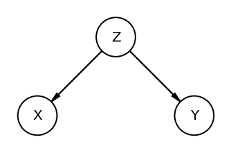
Fork is a classic confounder. Z is common cause of X & Y. Learning X tells us nothing about Y
The Pipe
dag_the_pipe = CausalGraphicalModel(
    nodes=["X", "Y", "Z"], edges=[("X", "Z"), ("Z", "Y")]
)

pgm = daft.PGM()
coordinates = {"X": (0, 0), "Y": (2, 0), "Z": (1, 0)}
for node in dag_the_pipe.dag.nodes:
    pgm.add_node(node, node, *coordinates[node])
for edge in dag_the_pipe.dag.edges:
    pgm.add_edge(*edge)
pgm.render();
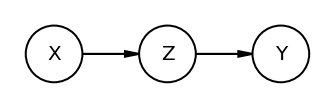
If we condition on Z we block the path from X to Y. Recall the treatment & fungus experiment
The Collider
dag_the_collider = CausalGraphicalModel(
    nodes=["X", "Y", "Z"], edges=[("X", "Z"), ("Y", "Z")]
)

pgm = daft.PGM()
coordinates = {"X": (0, 0), "Y": (2, 0), "Z": (1, 0)}
for node in dag_the_collider.dag.nodes:
    pgm.add_node(node, node, *coordinates[node])
for edge in dag_the_collider.dag.edges:
    pgm.add_edge(*edge)
pgm.render();
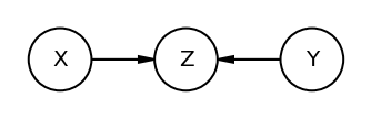
Conditioning on collider i.e Z opens the path i.e info flows between X and Y
The Descendant
dag_the_descendant = CausalGraphicalModel(
    nodes=["X", "Y", "Z", "D"], edges=[("X", "Z"), ("Y", "Z"), ("Z", "D")]
)

pgm = daft.PGM()
coordinates = {"X": (0, 1), "Y": (2, 1), "Z": (1, 0), "D": (1, -1)}
for node in dag_the_descendant.dag.nodes:
    pgm.add_node(node, node, *coordinates[node])
for edge in dag_the_descendant.dag.edges:
    pgm.add_edge(*edge)
pgm.render();
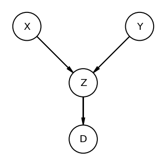
Here is D is the descendant variable. if we condition on it then it will be similar to closig the pipe.
6.4.2 Two roads
DAG shown below (Code 6.29) has U which is unobserved variable
We are interested in X->Y but which observed covariates (A, B, C) do we need to add to the model ?
Code 6.29
dag_6_1 = CausalGraphicalModel(
    nodes=["X", "Y", "C", "U", "B", "A"],
    edges=[
        ("X", "Y"),
        ("U", "X"),
        ("A", "U"),
        ("A", "C"),
        ("C", "Y"),
        ("U", "B"),
        ("C", "B"),
    ],
)


# let's render the DAG as well (note - no code section for it in the book but is displayed)
# so instead of copying the picture we are generating it
pgm = daft.PGM()
coordinates = {
    "X": (0, 3),
    "Y": (2, 3),
    "U": (0, 1),
    "C": (2, 1),
    "A": (1, 0),
    "B": (1, 2),
}
for node in dag_6_1.dag.nodes:
    pgm.add_node(node, node, *coordinates[node])
for edge in dag_6_1.dag.edges:
    pgm.add_edge(*edge)
pgm.render();
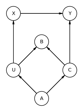
all_adjustment_sets = dag_6_1.get_all_backdoor_adjustment_sets("X", "Y")
for s in all_adjustment_sets:
    if all(not t.issubset(s) for t in all_adjustment_sets if t != s):
        if s != {"U"}:
            print(s)
frozenset({'A'})
frozenset({'C'})
Read above results as -
Conditioning on either A or C would suffice
6.4.3 Backdoor waffles
Let’s consider the Waffle House & Divorce rate correlation and with the help of graph we can find the covariates we should include in our model
Code 6.30
S => Whether or not state is in southern USA
A => Median Age
M => Marriage Rate
W => Number of Waffle Houses
D => Divorce Rate
dag_6_2 = CausalGraphicalModel(
    nodes=["S", "A", "D", "M", "W"],
    edges=[
        ("S", "A"),
        ("A", "D"),
        ("S", "M"),
        ("M", "D"),
        ("S", "W"),
        ("W", "D"),
        ("A", "M"),
    ],
)

# let's render the DAG as well (note - no code section for it in the book but is displayed)
# so instead of copying the picture we are generating it

pgm = daft.PGM()
coordinates = {
    "S": (0, 0),
    "W": (2, 0),
    "A": (0, 2),
    "D": (2, 2),
    "M": (1, 1),
}
for node in dag_6_2.dag.nodes:
    pgm.add_node(node, node, *coordinates[node])
for edge in dag_6_2.dag.edges:
    pgm.add_edge(*edge)
pgm.render();
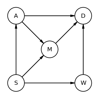
all_adjustment_sets = dag_6_2.get_all_backdoor_adjustment_sets("W", "D")
for s in all_adjustment_sets:
    if all(not t.issubset(s) for t in all_adjustment_sets if t != s):
        print(s)
frozenset({'A', 'M'})
frozenset({'S'})
This shows that we could control either for S alone or A and M
Code 6.31
Above DAG is not satisfactory as it assumes that there are no unobserved confounds.
We can further test the graph by finding the conditional independencies
all_independencies = dag_6_2.get_all_independence_relationships()
for s in all_independencies:
    if all(
        t[0] != s[0] or t[1] != s[1] or not t[2].issubset(s[2])
        for t in all_independencies
        if t != s
    ):
        print(s)
('A', 'W', {'S'})
('S', 'D', {'W', 'A', 'M'})
('M', 'W', {'S'})
Read above result as :
Marriage Rate & Waffle Houses should be independent if conditioning on S
Median Age & Waffle Houses should be independent if conditioning on S
Being in south and Divorce Rate should be indpendent if condition on (W, M and A)