.ipynb .pdf

repository open issue

Binder

Contents

8. Conditional Manatees

# Install packages that are not installed in colab
try:
  import google.colab
  %pip install -q watermark
  %pip install git+https://github.com/ksachdeva/rethinking-tensorflow-probability.git
except:
  pass

%load_ext watermark

# Core
import numpy as np
import arviz as az
import xarray as xr
import tensorflow as tf
import tensorflow_probability as tfp

# visualization
import matplotlib.pyplot as plt

from rethinking.data import RethinkingDataset
from rethinking.data import dataframe_to_tensors
from rethinking.mcmc import sample_posterior

# aliases
tfd = tfp.distributions
tfb = tfp.bijectors
Root = tfd.JointDistributionCoroutine.Root

2022-01-19 19:01:11.227162: W tensorflow/stream_executor/platform/default/dso_loader.cc:64] Could not load dynamic library 'libcudart.so.11.0'; dlerror: libcudart.so.11.0: cannot open shared object file: No such file or directory
2022-01-19 19:01:11.227210: I tensorflow/stream_executor/cuda/cudart_stub.cc:29] Ignore above cudart dlerror if you do not have a GPU set up on your machine.

%watermark -p numpy,tensorflow,tensorflow_probability,arviz,scipy,pandas

numpy                 : 1.21.5
tensorflow            : 2.7.0
tensorflow_probability: 0.15.0
arviz                 : 0.11.4
scipy                 : 1.7.3
pandas                : 1.3.5

# config of various plotting libraries
%config InlineBackend.figure_format = 'retina'

8.1 Building an interaction

8.1.1 Making a rugged model

Code 8.1

Every inference is conditional on something whether we notice it or not !

So far in the book, it was assumed that the predictor variable has an independent association with the mean of the outcome. What if want to allow the association to be conditional ?

d = RethinkingDataset.Rugged.get_dataset()

# make log version of outcome
d["log_gdp"] = d["rgdppc_2000"].pipe(np.log)

# extract countries with GDP data
dd = d[d["rgdppc_2000"].notnull()].copy()

# rescale variables
dd["log_gdp_std"] = dd.log_gdp / dd.log_gdp.mean()
dd["rugged_std"] = dd.rugged / dd.rugged.max()

# split countries into Africa and not-Africa
d_A1 = dd[dd["cont_africa"] == 1]  # Africa
d_A0 = dd[dd["cont_africa"] == 0]  # not Africa

Note - terrain ruggedness is divided by the maximum value observed

Code 8.2

def model_8_1(rugged_std):
    def _generator():
        alpha = yield Root(
            tfd.Sample(tfd.Normal(loc=1.0, scale=1.0, name="alpha"), sample_shape=1)
        )
        beta = yield Root(
            tfd.Sample(tfd.Normal(loc=0.0, scale=1.0, name="beta"), sample_shape=1)
        )
        sigma = yield Root(
            tfd.Sample(tfd.Exponential(rate=1.0, name="sigma"), sample_shape=1)
        )

        mu = alpha + beta * (rugged_std - 0.215)

        log_gdp_std = yield tfd.Independent(
            tfd.Normal(loc=mu, scale=sigma), reinterpreted_batch_ndims=1
        )

    return tfd.JointDistributionCoroutine(_generator, validate_args=False)

Code 8.3

jdc_8_1 = model_8_1(rugged_std=dd["rugged_std"].values)

sample_alpha, sample_beta, sample_sigma, _ = jdc_8_1.sample(1000)

# set up the plot dimensions
plt.subplot(xlim=(0, 1), ylim=(0.5, 1.5), xlabel="ruggedness", ylabel="log GDP")
plt.gca().axhline(dd.log_gdp_std.min(), ls="--")
plt.gca().axhline(dd.log_gdp_std.max(), ls="--")

# draw 50 lines from the prior
rugged_seq = np.linspace(-0.1, 1.1, num=30)

jdc_8_1_test = model_8_1(rugged_std=rugged_seq)

ds, _ = jdc_8_1_test.sample_distributions(
    value=[sample_alpha, sample_beta, sample_sigma, None]
)

mu = ds[-1].distribution.loc

for i in range(50):
    plt.plot(rugged_seq, mu[i], "k", alpha=0.3)

2022-01-19 19:01:14.138503: W tensorflow/stream_executor/platform/default/dso_loader.cc:64] Could not load dynamic library 'libcuda.so.1'; dlerror: libcuda.so.1: cannot open shared object file: No such file or directory
2022-01-19 19:01:14.138539: W tensorflow/stream_executor/cuda/cuda_driver.cc:269] failed call to cuInit: UNKNOWN ERROR (303)
2022-01-19 19:01:14.138564: I tensorflow/stream_executor/cuda/cuda_diagnostics.cc:156] kernel driver does not appear to be running on this host (fv-az272-145): /proc/driver/nvidia/version does not exist
2022-01-19 19:01:14.138788: I tensorflow/core/platform/cpu_feature_guard.cc:151] This TensorFlow binary is optimized with oneAPI Deep Neural Network Library (oneDNN) to use the following CPU instructions in performance-critical operations:  AVX2 FMA
To enable them in other operations, rebuild TensorFlow with the appropriate compiler flags.

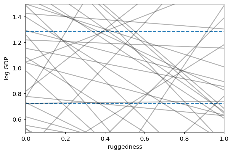
Code 8.4

np.sum(np.abs(sample_beta) > 0.6) / sample_beta.shape[0]

0.56

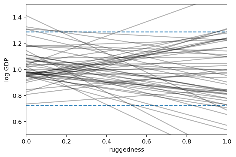
Code 8.5

tdf = dataframe_to_tensors("Rugged", dd, ["rugged_std", "log_gdp_std"])

def model_8_1(rugged_std):
    def _generator():
        alpha = yield Root(
            tfd.Sample(tfd.Normal(loc=1.0, scale=0.1, name="alpha"), sample_shape=1)
        )
        beta = yield Root(
            tfd.Sample(tfd.Normal(loc=0.0, scale=0.3, name="beta"), sample_shape=1)
        )
        sigma = yield Root(
            tfd.Sample(tfd.Exponential(rate=1.0, name="sigma"), sample_shape=1)
        )

        mu = alpha[..., tf.newaxis] + beta[..., tf.newaxis] * (rugged_std - 0.215)
        scale = sigma[..., tf.newaxis]

        log_gdp_std = yield tfd.Independent(
            tfd.Normal(loc=mu, scale=scale), reinterpreted_batch_ndims=1
        )

    return tfd.JointDistributionCoroutine(_generator, validate_args=False)


jdc_8_1 = model_8_1(tdf.rugged_std)

sample_alpha, sample_beta, sample_sigma, _ = jdc_8_1.sample(1000)

# set up the plot dimensions
plt.subplot(xlim=(0, 1), ylim=(0.5, 1.5), xlabel="ruggedness", ylabel="log GDP")
plt.gca().axhline(dd.log_gdp_std.min(), ls="--")
plt.gca().axhline(dd.log_gdp_std.max(), ls="--")

# draw 50 lines from the prior
rugged_seq = np.linspace(-0.1, 1.1, num=30)

jdc_8_1_test = model_8_1(rugged_std=rugged_seq)

ds, _ = jdc_8_1_test.sample_distributions(
    value=[sample_alpha, sample_beta, sample_sigma, None]
)

mu = tf.squeeze(ds[-1].distribution.loc)

for i in range(50):
    plt.plot(rugged_seq, mu[i], "k", alpha=0.3)

Code 8.6

NUM_CHAINS_FOR_8_1 = 2

init_state = [
    tf.ones([NUM_CHAINS_FOR_8_1]),
    tf.zeros([NUM_CHAINS_FOR_8_1]),
    tf.ones([NUM_CHAINS_FOR_8_1]),
]


bijectors = [
    tfb.Identity(),
    tfb.Identity(),
    tfb.Exp(),
]

posterior_8_1, trace_8_1 = sample_posterior(
    jdc_8_1,
    observed_data=(tdf.log_gdp_std,),
    params=["alpha", "beta", "sigma"],
    init_state=init_state,
    bijectors=bijectors,
)

az.summary(trace_8_1, hdi_prob=0.89)

	mean	sd	hdi_5.5%	hdi_94.5%	mcse_mean	mcse_sd	ess_bulk	ess_tail	r_hat
alpha	1.000	0.010	0.984	1.018	0.000	0.000	1028.0	433.0	1.00
beta	0.002	0.057	-0.078	0.093	0.003	0.002	278.0	416.0	1.02
sigma	0.138	0.008	0.125	0.149	0.000	0.000	372.0	288.0	1.00

8.1.2 Adding an indicator variable isn’t enough

Code 8.7

# make variable to index Africa (0) or not (1)
dd["cid"] = np.where(dd.cont_africa.values == 1, 0, 1)

dd["cid"]

2      0
4      1
7      1
8      1
9      1
      ..
229    1
230    1
231    0
232    0
233    0
Name: cid, Length: 170, dtype: int64

Code 8.8

tdf = dataframe_to_tensors(
    "Rugged", dd, {"rugged_std": tf.float32, "log_gdp_std": tf.float32, "cid": tf.int32}
)

def model_8_2(cid, rugged_std):
    def _generator():
        alpha = yield Root(
            tfd.Sample(tfd.Normal(loc=1.0, scale=0.1, name="alpha"), sample_shape=2)
        )
        beta = yield Root(
            tfd.Sample(tfd.Normal(loc=0.0, scale=0.3, name="beta"), sample_shape=1)
        )
        sigma = yield Root(
            tfd.Sample(tfd.Exponential(rate=1.0, name="sigma"), sample_shape=1)
        )

        mu = tf.gather(alpha, cid, axis=-1) + beta[..., tf.newaxis] * (
            rugged_std - 0.215
        )
        scale = sigma[..., tf.newaxis]

        log_gdp_std = yield tfd.Independent(
            tfd.Normal(loc=mu, scale=scale), reinterpreted_batch_ndims=1
        )

    return tfd.JointDistributionCoroutine(_generator, validate_args=False)


jdc_8_2 = model_8_2(tdf.cid, rugged_std=tdf.rugged_std)

NUMBER_OF_CHAINS = 2

init_state = [
    tf.ones([NUMBER_OF_CHAINS, 2]),
    tf.zeros([NUMBER_OF_CHAINS]),
    tf.ones([NUMBER_OF_CHAINS]),
]

bijectors = [
    tfb.Identity(),
    tfb.Identity(),
    tfb.Exp(),
]

posterior_8_2, trace_8_2 = sample_posterior(
    jdc_8_2,
    observed_data=(tdf.log_gdp_std,),
    params=["alpha", "beta", "sigma"],
    init_state=init_state,
    bijectors=bijectors,
)

az.summary(trace_8_2, hdi_prob=0.89)

	mean	sd	hdi_5.5%	hdi_94.5%	mcse_mean	mcse_sd	ess_bulk	ess_tail	r_hat
alpha[0]	0.881	0.016	0.852	0.905	0.000	0.000	1226.0	782.0	1.0
alpha[1]	1.050	0.010	1.035	1.066	0.001	0.000	285.0	268.0	1.0
beta	-0.047	0.048	-0.136	0.019	0.002	0.002	479.0	459.0	1.0
sigma	0.114	0.007	0.104	0.125	0.000	0.000	291.0	365.0	1.0

Code 8.9

def compute_and_store_log_likelihood_for_model_8_1():

    sample_alpha = posterior_8_1["alpha"]
    sample_beta = posterior_8_1["beta"]
    sample_sigma = posterior_8_1["sigma"]

    ds, _ = jdc_8_1.sample_distributions(
        value=[sample_alpha, sample_beta, sample_sigma, None]
    )

    log_likelihood_8_1 = ds[-1].distribution.log_prob(tdf.log_gdp_std).numpy()

    # we need to insert this in the sampler_stats
    sample_stats_8_1 = trace_8_1.sample_stats

    coords = [
        sample_stats_8_1.coords["chain"],
        sample_stats_8_1.coords["draw"],
        np.arange(170),
    ]

    sample_stats_8_1["log_likelihood"] = xr.DataArray(
        log_likelihood_8_1,
        coords=coords,
        dims=["chain", "draw", "log_likelihood_dim_0"],
    )


compute_and_store_log_likelihood_for_model_8_1()

# We need to first compute the log likelihoods so as to be able to compare them
def compute_and_store_log_likelihood_for_model_8_2():

    sample_alpha = posterior_8_2["alpha"]
    sample_beta = posterior_8_2["beta"]
    sample_sigma = posterior_8_2["sigma"]

    ds, _ = jdc_8_2.sample_distributions(
        value=[sample_alpha, sample_beta, sample_sigma, None]
    )

    log_likelihood_8_2 = ds[-1].distribution.log_prob(tdf.log_gdp_std).numpy()

    # we need to insert this in the sampler_stats
    sample_stats_8_2 = trace_8_2.sample_stats

    coords = [
        sample_stats_8_2.coords["chain"],
        sample_stats_8_2.coords["draw"],
        np.arange(170),
    ]

    sample_stats_8_2["log_likelihood"] = xr.DataArray(
        log_likelihood_8_2,
        coords=coords,
        dims=["chain", "draw", "log_likelihood_dim_0"],
    )


compute_and_store_log_likelihood_for_model_8_2()

az.compare({"m8.1": trace_8_1, "m8.2": trace_8_2})

	rank	loo	p_loo	d_loo	weight	se	dse	warning	loo_scale
m8.2	0	125.968312	4.329834	0.000000	0.964731	7.448146	0.000000	False	log
m8.1	1	94.428626	2.590254	31.539686	0.035269	6.506622	7.386764	False	log

Code 8.10

az.summary(trace_8_2, hdi_prob=0.89)

	mean	sd	hdi_5.5%	hdi_94.5%	mcse_mean	mcse_sd	ess_bulk	ess_tail	r_hat
alpha[0]	0.881	0.016	0.852	0.905	0.000	0.000	1226.0	782.0	1.0
alpha[1]	1.050	0.010	1.035	1.066	0.001	0.000	285.0	268.0	1.0
beta	-0.047	0.048	-0.136	0.019	0.002	0.002	479.0	459.0	1.0
sigma	0.114	0.007	0.104	0.125	0.000	0.000	291.0	365.0	1.0

Code 8.11

diff_a = trace_8_2.posterior["alpha"][:, :, 0] - trace_8_2.posterior["alpha"][:, :, 1]

trace_8_2.posterior["diff_a"] = diff_a

az.summary(trace_8_2, hdi_prob=0.89)

	mean	sd	hdi_5.5%	hdi_94.5%	mcse_mean	mcse_sd	ess_bulk	ess_tail	r_hat
alpha[0]	0.881	0.016	0.852	0.905	0.000	0.000	1226.0	782.0	1.0
alpha[1]	1.050	0.010	1.035	1.066	0.001	0.000	285.0	268.0	1.0
beta	-0.047	0.048	-0.136	0.019	0.002	0.002	479.0	459.0	1.0
sigma	0.114	0.007	0.104	0.125	0.000	0.000	291.0	365.0	1.0
diff_a	-0.169	0.019	-0.196	-0.135	0.001	0.001	639.0	624.0	1.0

Code 8.12

rugged_seq = np.linspace(start=-1, stop=1.1, num=30)

sample_alpha = posterior_8_2["alpha"][0]
sample_beta = posterior_8_2["beta"][0]
sample_sigma = posterior_8_2["sigma"][0]

# compute mu over samples, fixing cid=1
jdc_8_2_test_cid_1 = model_8_2(np.repeat(1, 30), rugged_std=rugged_seq)

ds, samples = jdc_8_2_test_cid_1.sample_distributions(
    value=[sample_alpha, sample_beta, sample_sigma, None]
)

mu_NotAfrica = tf.squeeze(ds[-1].distribution.loc)
mu_NotAfrica_mu = tf.reduce_mean(mu_NotAfrica, 0)
mu_NotAfrica_ci = tfp.stats.percentile(mu_NotAfrica, q=(1.5, 98.5), axis=0)

# compute mu over samples, fixing cid=0
jdc_8_2_test_cid_0 = model_8_2(np.repeat(0, 30), rugged_std=rugged_seq)

ds, samples = jdc_8_2_test_cid_0.sample_distributions(
    value=[sample_alpha, sample_beta, sample_sigma, None]
)

mu_Africa = tf.squeeze(ds[-1].distribution.loc)
mu_Africa_mu = tf.reduce_mean(mu_Africa, 0)
mu_Africa_ci = tfp.stats.percentile(mu_Africa, q=(1.5, 98.5), axis=0)

# draw figure 8.4 in the book [note - no code was provided for it in the book]

plt.xlim(0.0, 1.0)
plt.scatter(
    dd.rugged_std,
    dd.log_gdp_std,
    edgecolors=["none" if i == 0 else "b" for i in dd["cid"]],
    facecolors=["none" if i == 1 else "b" for i in dd["cid"]],
)

# draw MAP line
plt.plot(rugged_seq, mu_Africa_mu, "b", label="Africa")
plt.fill_between(rugged_seq, mu_Africa_ci[0], mu_Africa_ci[1], color="b", alpha=0.2)

plt.plot(rugged_seq, mu_NotAfrica_mu, "k", label="Not Africa")
plt.fill_between(
    rugged_seq, mu_NotAfrica_ci[0], mu_NotAfrica_ci[1], color="k", alpha=0.2
)

plt.legend();

Code 8.13

def model_8_3(cid, rugged_std):
    def _generator():
        alpha = yield Root(
            tfd.Sample(tfd.Normal(loc=1.0, scale=0.1, name="alpha"), sample_shape=2)
        )
        beta = yield Root(
            tfd.Sample(tfd.Normal(loc=0.0, scale=0.3, name="beta"), sample_shape=2)
        )
        sigma = yield Root(
            tfd.Sample(tfd.Exponential(rate=1.0, name="sigma"), sample_shape=1)
        )

        mu = tf.gather(alpha, cid, axis=-1) + tf.gather(beta, cid, axis=-1) * (
            rugged_std - 0.215
        )
        scale = sigma[..., tf.newaxis]

        log_gdp_std = yield tfd.Independent(
            tfd.Normal(loc=mu, scale=scale), reinterpreted_batch_ndims=1
        )

    return tfd.JointDistributionCoroutine(_generator, validate_args=False)


jdc_8_3 = model_8_3(tdf.cid, rugged_std=tdf.rugged_std)

init_state = [
    tf.ones([NUMBER_OF_CHAINS, 2]),
    tf.zeros([NUMBER_OF_CHAINS, 2]),
    tf.ones([NUMBER_OF_CHAINS]),
]

bijectors = [
    tfb.Identity(),
    tfb.Identity(),
    tfb.Exp(),
]

posterior_8_3, trace_8_3 = sample_posterior(
    jdc_8_3,
    observed_data=(tdf.log_gdp_std,),
    params=["alpha", "beta", "sigma"],
    num_samples=1000,
    init_state=init_state,
    bijectors=bijectors,
)

Code 8.14

az.summary(trace_8_3, hdi_prob=0.89)

	mean	sd	hdi_5.5%	hdi_94.5%	mcse_mean	mcse_sd	ess_bulk	ess_tail	r_hat
alpha[0]	0.886	0.016	0.861	0.911	0.000	0.000	2375.0	1378.0	1.00
alpha[1]	1.050	0.010	1.036	1.067	0.000	0.000	431.0	587.0	1.01
beta[0]	0.133	0.079	0.008	0.256	0.005	0.004	239.0	464.0	1.01
beta[1]	-0.144	0.055	-0.230	-0.062	0.002	0.002	582.0	892.0	1.00
sigma	0.111	0.006	0.101	0.120	0.000	0.000	522.0	614.0	1.01

Code 8.15

# We need to first compute the log likelihoods so as to be able to compare them
def compute_and_store_log_likelihood_for_model_8_3():

    sample_alpha = posterior_8_3["alpha"]
    sample_beta = posterior_8_3["beta"]
    sample_sigma = posterior_8_3["sigma"]

    ds, _ = jdc_8_3.sample_distributions(
        value=[sample_alpha, sample_beta, sample_sigma, None]
    )

    log_likelihood_8_3 = ds[-1].distribution.log_prob(tdf.log_gdp_std).numpy()

    # we need to insert this in the sampler_stats
    sample_stats_8_3 = trace_8_3.sample_stats

    coords = [
        sample_stats_8_3.coords["chain"],
        sample_stats_8_3.coords["draw"],
        np.arange(170),
    ]

    sample_stats_8_3["log_likelihood"] = xr.DataArray(
        log_likelihood_8_3,
        coords=coords,
        dims=["chain", "draw", "log_likelihood_dim_0"],
    )


compute_and_store_log_likelihood_for_model_8_3()

az.compare({"m8.1": trace_8_1, "m8.2": trace_8_2, "m8.3": trace_8_3})

	rank	loo	p_loo	d_loo	weight	se	dse	warning	loo_scale
m8.3	0	129.606079	5.002433	0.000000	8.738141e-01	7.358786	0.000000	False	log
m8.2	1	125.968900	4.329246	3.637179	1.261859e-01	7.448509	3.310409	False	log
m8.1	2	94.428626	2.590254	35.177453	4.440892e-16	6.506622	7.503596	False	log

Code 8.16

az.waic(trace_8_3, pointwise=True)

/opt/hostedtoolcache/Python/3.7.12/x64/lib/python3.7/site-packages/arviz/stats/stats.py:1460: UserWarning: For one or more samples the posterior variance of the log predictive densities exceeds 0.4. This could be indication of WAIC starting to fail. 
See http://arxiv.org/abs/1507.04544 for details
  "For one or more samples the posterior variance of the log predictive "

Computed from 2000 by 170 log-likelihood matrix

          Estimate       SE
elpd_waic   129.67     7.35
p_waic        4.94        -

There has been a warning during the calculation. Please check the results.

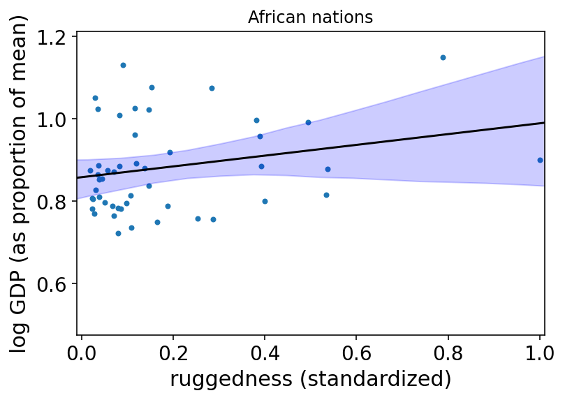
8.1.4 Plotting the interaction

Code 8.17

rugged_seq = np.linspace(start=-1, stop=1.1, num=30)

sample_alpha = posterior_8_3["alpha"][0]
sample_beta = posterior_8_3["beta"][0]
sample_sigma = posterior_8_3["sigma"][0]

# compute mu over samples, fixing cid=1
jdc_8_3_test_cid_1 = model_8_3(np.repeat(1, 30), rugged_std=rugged_seq)

ds, samples = jdc_8_3_test_cid_1.sample_distributions(
    value=[sample_alpha, sample_beta, sample_sigma, None]
)

mu_NotAfrica = tf.squeeze(ds[-1].distribution.loc)
mu_NotAfrica_mu = tf.reduce_mean(mu_NotAfrica, 0)
mu_NotAfrica_ci = tfp.stats.percentile(mu_NotAfrica, q=(1.5, 98.5), axis=0)

# compute mu over samples, fixing cid=0
jdc_8_3_test_cid_0 = model_8_3(np.repeat(0, 30), rugged_std=rugged_seq)

ds, samples = jdc_8_3_test_cid_0.sample_distributions(
    value=[sample_alpha, sample_beta, sample_sigma, None]
)

mu_Africa = tf.squeeze(ds[-1].distribution.loc)
mu_Africa_mu = tf.reduce_mean(mu_Africa, 0)
mu_Africa_ci = tfp.stats.percentile(mu_Africa, q=(1.5, 98.5), axis=0)

az.plot_pair(d_A1[["rugged_std", "log_gdp_std"]].to_dict(orient="list"))
plt.gca().set(
    xlim=(-0.01, 1.01),
    xlabel="ruggedness (standardized)",
    ylabel="log GDP (as proportion of mean)",
)

plt.plot(rugged_seq, mu_Africa_mu, "k")
plt.fill_between(rugged_seq, mu_Africa_ci[0], mu_Africa_ci[1], color="b", alpha=0.2)
plt.title("African nations")
plt.show();

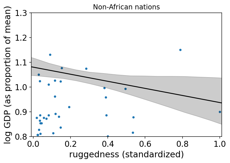
az.plot_pair(d_A1[["rugged_std", "log_gdp_std"]].to_dict(orient="list"))
plt.gca().set(
    xlim=(-0.01, 1.01),
    xlabel="ruggedness (standardized)",
    ylim=(0.8, 1.3),
    ylabel="log GDP (as proportion of mean)",
)

plt.plot(rugged_seq, mu_NotAfrica_mu, "k")
plt.fill_between(
    rugged_seq, mu_NotAfrica_ci[0], mu_NotAfrica_ci[1], color="k", alpha=0.2
)
plt.title("Non-African nations")
plt.show()

8.2 Symmetry of interactions

Code 8.18

# TODO - draw corresponding graph (Figure 8.6)

rugged_seq = np.linspace(start=-0.2, stop=1.2, num=30)
delta = mu_Africa_mu - mu_NotAfrica_mu

8.3 Continuous interactions

8.3.1 A winter flower

Code 8.19

d = RethinkingDataset.Tulips.get_dataset()
d.info()
d.head()

<class 'pandas.core.frame.DataFrame'>
RangeIndex: 27 entries, 0 to 26
Data columns (total 4 columns):
 #   Column  Non-Null Count  Dtype  
---  ------  --------------  -----  
 0   bed     27 non-null     object 
 1   water   27 non-null     int64  
 2   shade   27 non-null     int64  
 3   blooms  27 non-null     float64
dtypes: float64(1), int64(2), object(1)
memory usage: 992.0+ bytes

	bed	water	shade	blooms
0	a	1	1	0.00
1	a	1	2	0.00
2	a	1	3	111.04
3	a	2	1	183.47
4	a	2	2	59.16

Code 8.20

d["blooms_std"] = d.blooms / d.blooms.max()
d["water_cent"] = d.water - d.water.mean()
d["shade_cent"] = d.shade - d.shade.mean()

Code 8.21

a = tfd.Normal(loc=0.5, scale=1.0).sample((int(1e4),))
np.sum((a < 0) | (a > 1)) / a.shape[0]

0.6196

Code 8.22

a = tfd.Normal(loc=0.5, scale=0.25).sample((int(1e4),))
np.sum((a < 0) | (a > 1)) / a.shape[0]

0.0497

Code 8.23

tdf = dataframe_to_tensors("Tulip", d, ["blooms_std", "water_cent", "shade_cent"])

def model_8_4(
    water_cent,
    shade_cent,
):
    def _generator():
        alpha = yield Root(
            tfd.Sample(tfd.Normal(loc=0.5, scale=0.25, name="alpha"), sample_shape=1)
        )
        betaW = yield Root(
            tfd.Sample(tfd.Normal(loc=0.0, scale=0.25, name="betaW"), sample_shape=1)
        )
        betaS = yield Root(
            tfd.Sample(tfd.Normal(loc=0.0, scale=0.25, name="betaS"), sample_shape=1)
        )
        sigma = yield Root(
            tfd.Sample(tfd.Exponential(rate=1.0, name="sigma"), sample_shape=1)
        )

        mu = (
            alpha[..., tf.newaxis]
            + betaW[..., tf.newaxis] * water_cent
            + betaS[..., tf.newaxis] * shade_cent
        )
        scale = sigma[..., tf.newaxis]

        log_gdp_std = yield tfd.Independent(
            tfd.Normal(loc=mu, scale=scale), reinterpreted_batch_ndims=1
        )

    return tfd.JointDistributionCoroutine(_generator, validate_args=False)


jdc_8_4 = model_8_4(shade_cent=tdf.shade_cent, water_cent=tdf.water_cent)

init_state = [
    0.5 * tf.ones([NUMBER_OF_CHAINS]),
    tf.zeros([NUMBER_OF_CHAINS]),
    tf.zeros([NUMBER_OF_CHAINS]),
    tf.ones([NUMBER_OF_CHAINS]),
]

bijectors = [
    tfb.Identity(),
    tfb.Identity(),
    tfb.Identity(),
    tfb.Exp(),
]

posterior_8_4, trace_8_4 = sample_posterior(
    jdc_8_4,
    observed_data=(tdf.blooms_std,),
    params=["alpha", "betaW", "betaS", "sigma"],
    num_samples=1000,
    init_state=init_state,
    bijectors=bijectors,
)

Code 8.24

def model_8_5(water_cent, shade_cent):
    def _generator():
        alpha = yield Root(
            tfd.Sample(tfd.Normal(loc=0.5, scale=0.25, name="alpha"), sample_shape=1)
        )
        betaW = yield Root(
            tfd.Sample(tfd.Normal(loc=0.0, scale=0.25, name="betaW"), sample_shape=1)
        )
        betaS = yield Root(
            tfd.Sample(tfd.Normal(loc=0.0, scale=0.25, name="betaS"), sample_shape=1)
        )
        betaWS = yield Root(
            tfd.Sample(tfd.Normal(loc=0.0, scale=0.25, name="betaWS"), sample_shape=1)
        )
        sigma = yield Root(
            tfd.Sample(tfd.Exponential(rate=1.0, name="sigma"), sample_shape=1)
        )

        mu = (
            alpha[..., tf.newaxis]
            + betaW[..., tf.newaxis] * water_cent
            + betaS[..., tf.newaxis] * shade_cent
            + betaWS[..., tf.newaxis] * shade_cent * water_cent
        )

        scale = sigma[..., tf.newaxis]

        log_gdp_std = yield tfd.Independent(
            tfd.Normal(loc=mu, scale=scale), reinterpreted_batch_ndims=1
        )

    return tfd.JointDistributionCoroutine(_generator, validate_args=False)


jdc_8_5 = model_8_5(shade_cent=tdf.shade_cent, water_cent=tdf.water_cent)

init_state = [
    0.5 * tf.ones([NUMBER_OF_CHAINS]),
    tf.zeros([NUMBER_OF_CHAINS]),
    tf.zeros([NUMBER_OF_CHAINS]),
    tf.zeros([NUMBER_OF_CHAINS]),
    tf.ones([NUMBER_OF_CHAINS]),
]

bijectors = [
    tfb.Identity(),
    tfb.Identity(),
    tfb.Identity(),
    tfb.Identity(),
    tfb.Exp(),
]

posterior_8_5, trace_8_5 = sample_posterior(
    jdc_8_5,
    observed_data=(tdf.blooms_std,),
    params=["alpha", "betaW", "betaS", "betaWS", "sigma"],
    num_samples=1000,
    init_state=init_state,
    bijectors=bijectors,
)

WARNING:tensorflow:5 out of the last 5 calls to <function run_hmc_chain at 0x7fb05a5af7a0> triggered tf.function retracing. Tracing is expensive and the excessive number of tracings could be due to (1) creating @tf.function repeatedly in a loop, (2) passing tensors with different shapes, (3) passing Python objects instead of tensors. For (1), please define your @tf.function outside of the loop. For (2), @tf.function has experimental_relax_shapes=True option that relaxes argument shapes that can avoid unnecessary retracing. For (3), please refer to https://www.tensorflow.org/guide/function#controlling_retracing and https://www.tensorflow.org/api_docs/python/tf/function for  more details.

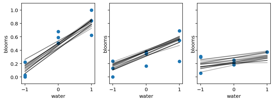
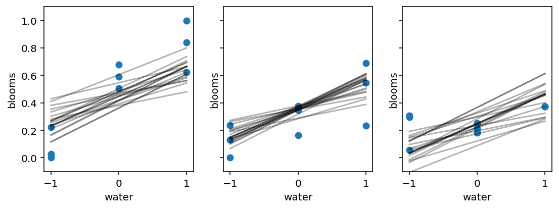
8.3.3 Plotting posterior predictions

Code 8.25

sample_alpha = posterior_8_4["alpha"][0]
sample_betaW = posterior_8_4["betaW"][0]
sample_betaS = posterior_8_4["betaS"][0]
sample_sigma = posterior_8_4["sigma"][0]

_, axes = plt.subplots(1, 3, figsize=(9, 3), sharey=True)  # 3 plots in 1 row
for ax, s in zip(axes, range(-1, 2)):
    idx = d.shade_cent == s
    ax.scatter(d.water_cent[idx], d.blooms_std[idx])
    ax.set(xlim=(-1.1, 1.1), ylim=(-0.1, 1.1), xlabel="water", ylabel="blooms")

    shade_cent = s
    water_cent = np.arange(-1, 2)

    jdc_8_4_test = model_8_4(
        water_cent=tf.cast(water_cent, dtype=tf.float32),
        shade_cent=tf.cast(shade_cent, dtype=tf.float32),
    )

    ds, _ = jdc_8_4_test.sample_distributions(
        value=[sample_alpha, sample_betaW, sample_betaS, sample_sigma, None]
    )

    mu = tf.squeeze(ds[-1].distribution.loc)

    for i in range(20):
        ax.plot(range(-1, 2), mu[i], "k", alpha=0.3)

# Code for plotting model 8.5 is not listed in the book but there are corresponding figures so
# draw them here

sample_alpha = posterior_8_5["alpha"][0]
sample_betaW = posterior_8_5["betaW"][0]
sample_betaS = posterior_8_5["betaS"][0]
sample_betaWS = posterior_8_5["betaWS"][0]
sample_sigma = posterior_8_5["sigma"][0]

_, axes = plt.subplots(1, 3, figsize=(9, 3), sharey=True)  # 3 plots in 1 row
for ax, s in zip(axes, range(-1, 2)):
    idx = d.shade_cent == s
    ax.scatter(d.water_cent[idx], d.blooms_std[idx])
    ax.set(xlim=(-1.1, 1.1), ylim=(-0.1, 1.1), xlabel="water", ylabel="blooms")

    shade_cent = s
    water_cent = np.arange(-1, 2)

    jdc_8_5_test = model_8_5(
        water_cent=tf.cast(water_cent, dtype=tf.float32),
        shade_cent=tf.cast(shade_cent, dtype=tf.float32),
    )

    ds, _ = jdc_8_5_test.sample_distributions(
        value=[
            sample_alpha,
            sample_betaW,
            sample_betaS,
            sample_betaWS,
            sample_sigma,
            None,
        ]
    )

    mu = tf.squeeze(ds[-1].distribution.loc)

    for i in range(20):
        ax.plot(range(-1, 2), mu[i], "k", alpha=0.3)

8.3.4 Plotting prior predictions

Code 8.26

# prior for 8.5
prior_8_5 = jdc_8_5.sample(1000)

previous

7. Ulysses’ Compass

next

9. Markov Chain Monte Carlo