2. Small Worlds and Large Worlds
Contents
![]()
2. Small Worlds and Large Worlds
# Install packages that are not installed in colab
try:
  import google.colab
  !pip install watermark
except:
  pass
%load_ext watermark
# Core
import numpy as np
import arviz as az
import tensorflow as tf
import tensorflow_probability as tfp
import scipy.stats as stats

# visualization
import matplotlib.pyplot as plt

# aliases
tfd = tfp.distributions
2022-01-19 18:53:22.017922: W tensorflow/stream_executor/platform/default/dso_loader.cc:64] Could not load dynamic library 'libcudart.so.11.0'; dlerror: libcudart.so.11.0: cannot open shared object file: No such file or directory
2022-01-19 18:53:22.018005: I tensorflow/stream_executor/cuda/cudart_stub.cc:29] Ignore above cudart dlerror if you do not have a GPU set up on your machine.
%watermark -p numpy,tensorflow,tensorflow_probability,arviz,scipy,pandas
numpy                 : 1.21.5
tensorflow            : 2.7.0
tensorflow_probability: 0.15.0
arviz                 : 0.11.4
scipy                 : 1.7.3
pandas                : 1.3.5
# config of various plotting libraries
%config InlineBackend.figure_format = 'retina'
2.1 The garden of forking data
2.1.3 From counts to probability
Suppose we have a bag of four marbles, each of which can be either blue or white. There are five possible compositions of the bag, ranging from all white marbles to all blue marbles. Now, suppose we make three draws with replacement from the bag, and end up with blue, then white, then blue. If we were to count the ways that each bag composition could produce this combination of samples, we would find the vector in ways below. For example, there are zero ways that four white marbles could lead to this sample, three ways that a bag composition of one blue marble and three white marbles could lead to the sample, as so on.
We can convert these counts to probabilities by simply dividing the counts by the sum of all the counts.
Code 2.1
ways = tf.constant([0.0, 3, 8, 9, 0])
new_ways = ways / tf.reduce_sum(ways)

new_ways
2022-01-19 18:53:24.540624: W tensorflow/stream_executor/platform/default/dso_loader.cc:64] Could not load dynamic library 'libcuda.so.1'; dlerror: libcuda.so.1: cannot open shared object file: No such file or directory
2022-01-19 18:53:24.540666: W tensorflow/stream_executor/cuda/cuda_driver.cc:269] failed call to cuInit: UNKNOWN ERROR (303)
2022-01-19 18:53:24.540689: I tensorflow/stream_executor/cuda/cuda_diagnostics.cc:156] kernel driver does not appear to be running on this host (fv-az272-145): /proc/driver/nvidia/version does not exist
2022-01-19 18:53:24.541033: I tensorflow/core/platform/cpu_feature_guard.cc:151] This TensorFlow binary is optimized with oneAPI Deep Neural Network Library (oneDNN) to use the following CPU instructions in performance-critical operations:  AVX2 FMA
To enable them in other operations, rebuild TensorFlow with the appropriate compiler flags.
<tf.Tensor: shape=(5,), dtype=float32, numpy=array([0. , 0.15, 0.4 , 0.45, 0. ], dtype=float32)>
2.3 Components of the model
2.3.2.1 Observed variables
Consider a globe of the earth that we toss into the air nine times. We want to compute the probability that our right index finger will land on water six times out of nine. We can use the binomial distribution to compute this, using a probability of 0.5 of landing on water on each toss.
Code 2.2
tf.exp(tfd.Binomial(total_count=9, probs=0.5).log_prob(6))
WARNING:tensorflow:@custom_gradient grad_fn has 'variables' in signature, but no ResourceVariables were used on the forward pass.
<tf.Tensor: shape=(), dtype=float32, numpy=0.16406254>
2.4 Making the model go
2.4.3 Grid Approximation
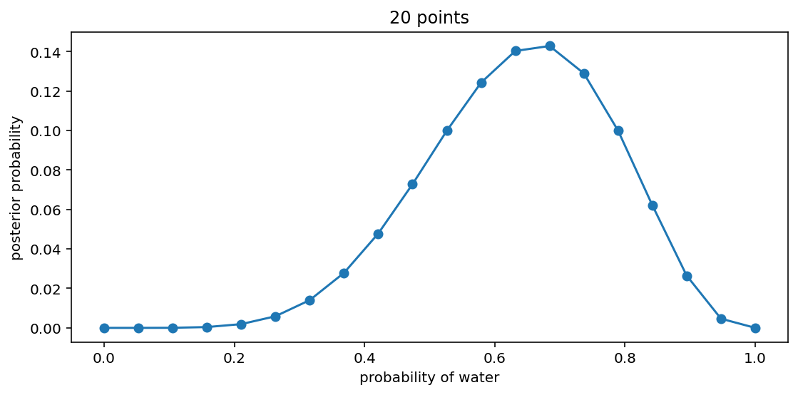
Create a grid approximation for the globe tossing model, for the scenario described in the section above. In the grid approximation technique, we approximate a continuous posterior distribution by using a discrete grid of parameter values.
Code 2.3
# define grid
n_points = 20  # change to an odd number for Code 2.5 graphs to
# match book examples in Figure 2.6
p_grid = tf.linspace(start=0.0, stop=1.0, num=n_points)

# define prior
prior = tf.ones([n_points])

# compute likelihood at each value in grid
likelihood = tfd.Binomial(total_count=9, probs=p_grid).prob(6)

# compute product of likelihood and prior
unstd_posterior = likelihood * prior

# standardize the posterior, so it sums to 1
posterior = unstd_posterior / tf.reduce_sum(unstd_posterior)

posterior
<tf.Tensor: shape=(20,), dtype=float32, numpy=
array([0.00000000e+00, 7.98984274e-07, 4.30771906e-05, 4.09079541e-04,
       1.89388765e-03, 5.87387430e-03, 1.40429335e-02, 2.78517436e-02,
       4.78011407e-02, 7.28073791e-02, 9.98729542e-02, 1.24264322e-01,
       1.40314341e-01, 1.42834887e-01, 1.28943324e-01, 9.98729020e-02,
       6.20589107e-02, 2.64547635e-02, 4.65966761e-03, 0.00000000e+00],
      dtype=float32)>
Code 2.4
_, ax = plt.subplots(figsize=(9, 4))
ax.plot(p_grid, posterior, "-o")
ax.set(xlabel="probability of water", ylabel="posterior probability", title="20 points");
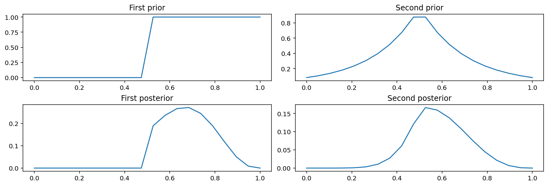
Code 2.5
first_prior = tf.where(condition=p_grid < 0.5, x=0.0, y=1)
second_prior = tf.exp(-5 * abs(p_grid - 0.5))

_, axes = plt.subplots(nrows=2, ncols=2, figsize=(12, 4), constrained_layout=True)

axes[0, 0].plot(p_grid, first_prior)
axes[0, 0].set_title("First prior")
axes[1, 0].plot(p_grid, first_prior * likelihood)
axes[1, 0].set_title("First posterior")

axes[0, 1].plot(p_grid, second_prior)
axes[0, 1].set_title("Second prior")
axes[1, 1].plot(p_grid, second_prior * likelihood)
axes[1, 1].set_title("Second posterior");
2.4.4 Quadratic Approximation
Code 2.6
TFP doesn’t natively provide a quap function, like in the book. But it has a lot of optimization tools. We’ll use bfgs, which gives us a somewhat straightforward way to get both the measurement and the standard error.
W = 6
L = 3
dist = tfd.JointDistributionNamed(
    {
        "water": lambda probability: tfd.Binomial(total_count=W + L, probs=probability),
        "probability": tfd.Uniform(low=0.0, high=1.0),
    }
)


def neg_log_prob(x):
    return tfp.math.value_and_gradient(
        lambda p: -dist.log_prob(
            water=W, probability=tf.clip_by_value(p[-1], 0.0, 1.0)
        ),
        x,
    )


results = tfp.optimizer.bfgs_minimize(neg_log_prob, initial_position=[0.5])
assert results.converged
The results object itself has a lot of information about the optimization process. The estimate is called the position, and we get the standard error from the inverse_hessian_estimate.
approximate_posterior = tfd.Normal(
    results.position,
    tf.sqrt(results.inverse_hessian_estimate),
)

print(
    "mean:",
    approximate_posterior.mean(),
    "\nstandard deviation: ",
    approximate_posterior.stddev(),
)
mean: tf.Tensor([[0.6666667]], shape=(1, 1), dtype=float32)
standard deviation:  tf.Tensor([[0.15718359]], shape=(1, 1), dtype=float32)
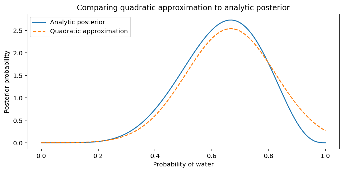
Let’s compare the mean and standard deviation from the quadratic approximation with an analytical approach based on the Beta distribution.
Code 2.7
_, ax = plt.subplots(figsize=(9, 4))

x = tf.linspace(0.0, 1.0, num=101)
ax.plot(x, tfd.Beta(W + 1, L + 1).prob(x), label="Analytic posterior")
# values obained from quadratic approximation
ax.plot(
    x, tf.squeeze(approximate_posterior.prob(x)), "--", label="Quadratic approximation"
)

ax.set(
    xlabel="Probability of water",
    ylabel="Posterior probability",
    title="Comparing quadratic approximation to analytic posterior",
)
ax.legend();
2.4.5. Markov chain Monte Carlo
We can estimate the posterior using a Markov chain Monte Carlo (MCMC) technique, which will be explained further in Chapter 9. An outline of the algorithm follows. It is written primarily in numpy to illustrate the steps you would take.
Code 2.8
n_samples = 1000
p = np.zeros(n_samples)
p[0] = 0.5
W = 6
L = 3
for i in range(1, n_samples):
    p_new = tfd.Normal(loc=p[i - 1], scale=0.1).sample(1)
    if p_new < 0:
        p_new = p_new
    if p_new > 1:
        p_new = 2 - p_new
    q0 = tf.exp(tfd.Binomial(total_count=W + L, probs=p[i - 1]).log_prob(W))
    q1 = tf.exp(tfd.Binomial(total_count=W + L, probs=p_new).log_prob(W))
    if stats.uniform.rvs(0, 1) < q1 / q0:
        p[i] = p_new
    else:
        p[i] = p[i - 1]
WARNING:tensorflow:@custom_gradient grad_fn has 'variables' in signature, but no ResourceVariables were used on the forward pass.
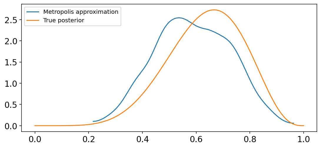
Code 2.9
With the samples from the posterior distribution in p, we can compare the results of the MCMC approximation to the analytical posterior.
_, ax = plt.subplots(figsize=(9, 4))

az.plot_kde(p, label="Metropolis approximation", ax=ax)
x = tf.linspace(0.0, 1.0, num=100)
ax.plot(x, tfd.Beta(W + 1, L + 1).prob(x), "C1", label="True posterior")
ax.legend();