12. Monsters and Mixtures¶

# Install packages that are not installed in colab
try:
  import google.colab
  %pip install -q watermark
  %pip install git+https://github.com/ksachdeva/rethinking-tensorflow-probability.git
except:
  pass

%load_ext watermark

# Core
import numpy as np
import arviz as az
import tensorflow as tf
import tensorflow_probability as tfp

# visualization
import matplotlib.pyplot as plt

from rethinking.data import RethinkingDataset
from rethinking.data import dataframe_to_tensors
from rethinking.mcmc import sample_posterior


# aliases
tfd = tfp.distributions
tfb = tfp.bijectors
Root = tfd.JointDistributionCoroutine.Root

2022-01-19 19:13:11.706740: W tensorflow/stream_executor/platform/default/dso_loader.cc:64] Could not load dynamic library 'libcudart.so.11.0'; dlerror: libcudart.so.11.0: cannot open shared object file: No such file or directory
2022-01-19 19:13:11.706778: I tensorflow/stream_executor/cuda/cudart_stub.cc:29] Ignore above cudart dlerror if you do not have a GPU set up on your machine.

%watermark -p numpy,tensorflow,tensorflow_probability,arviz,scipy,pandas,rethinking

numpy                 : 1.21.5
tensorflow            : 2.7.0
tensorflow_probability: 0.15.0
arviz                 : 0.11.4
scipy                 : 1.7.3
pandas                : 1.3.5
rethinking            : 0.1.0

# config of various plotting libraries
%config InlineBackend.figure_format = 'retina'

12.1 Over-dispersed counts¶

12.1.1 Beta-binomial¶

Code 12.1¶

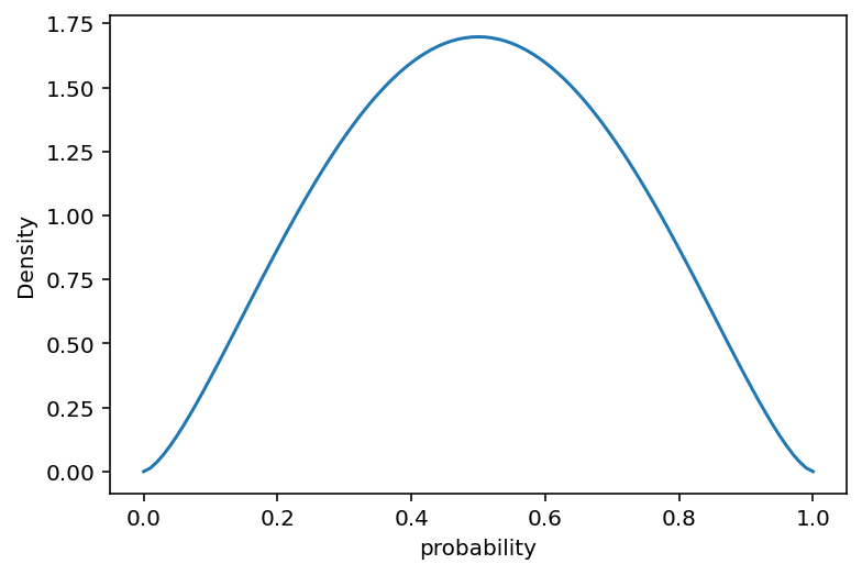
A beta distribution is a probability distribution for probabilities !

pbar = 0.5  # mean
theta = 5  # total concentration

alpha = pbar * theta
beta = (1 - pbar) * theta

x = np.linspace(0, 1, 101)

plt.plot(x, tf.exp(tfd.Beta(alpha, beta).log_prob(x)))
plt.gca().set(xlabel="probability", ylabel="Density")
plt.show()

WARNING:tensorflow:@custom_gradient grad_fn has 'variables' in signature, but no ResourceVariables were used on the forward pass.

2022-01-19 19:13:14.263744: W tensorflow/stream_executor/platform/default/dso_loader.cc:64] Could not load dynamic library 'libcuda.so.1'; dlerror: libcuda.so.1: cannot open shared object file: No such file or directory
2022-01-19 19:13:14.263785: W tensorflow/stream_executor/cuda/cuda_driver.cc:269] failed call to cuInit: UNKNOWN ERROR (303)
2022-01-19 19:13:14.263812: I tensorflow/stream_executor/cuda/cuda_diagnostics.cc:156] kernel driver does not appear to be running on this host (fv-az272-145): /proc/driver/nvidia/version does not exist
2022-01-19 19:13:14.264123: I tensorflow/core/platform/cpu_feature_guard.cc:151] This TensorFlow binary is optimized with oneAPI Deep Neural Network Library (oneDNN) to use the following CPU instructions in performance-critical operations:  AVX2 FMA
To enable them in other operations, rebuild TensorFlow with the appropriate compiler flags.

../_images/12_monsters_and_mixtures_10_2.png

Code 12.2¶

d = RethinkingDataset.UCBadmit.get_dataset()
d["gid"] = (d["applicant.gender"] != "male").astype(int)

tdf = dataframe_to_tensors(
    "UCBAdmit",
    d,
    {
        "gid": tf.int32,
        "applications": tf.float32,
        "admit": tf.float32,
        "reject": tf.float32,
    },
)

def model_12_1(gid, N):
    def _generator():
        alpha = yield Root(tfd.Sample(tfd.Normal(loc=0.0, scale=1.5), sample_shape=2))
        phi = yield Root(tfd.Sample(tfd.Exponential(rate=1.0), sample_shape=1))
        theta = phi + 2
        pbar = tf.sigmoid(tf.squeeze(tf.gather(alpha, gid, axis=-1)))

        # prepare the concentration vector
        concentration1 = pbar * theta[..., tf.newaxis]
        concentration0 = (1 - pbar) * theta[..., tf.newaxis]

        concentration = tf.stack([concentration1, concentration0], axis=-1)

        # outcome A i.e. admit
        # since it is a multinomial we will have K = 2
        # note -  this does not really behave like Binomial in terms of the sample shape
        A = yield tfd.Independent(
            tfd.DirichletMultinomial(total_count=N, concentration=concentration),
            reinterpreted_batch_ndims=1,
        )

    return tfd.JointDistributionCoroutine(_generator, validate_args=False)


jdc_12_1 = model_12_1(tdf.gid, tdf.applications)

Code 12.3¶

# Prepare the expected shape by the DirichletMultinomial
obs_values = tf.stack([tdf.admit, tdf.reject], axis=-1)

NUMBER_OF_CHAINS_12_1 = 2

init_state = [tf.zeros([NUMBER_OF_CHAINS_12_1, 2]), tf.ones([NUMBER_OF_CHAINS_12_1])]

bijectors = [tfb.Identity(), tfb.Identity()]


posterior_12_1, trace_12_1 = sample_posterior(
    jdc_12_1,
    num_samples=1000,
    observed_data=(obs_values,),
    init_state=init_state,
    bijectors=bijectors,
    params=["alpha", "phi"],
)

WARNING:tensorflow:@custom_gradient grad_fn has 'variables' in signature, but no ResourceVariables were used on the forward pass.

WARNING:tensorflow:@custom_gradient grad_fn has 'variables' in signature, but no ResourceVariables were used on the forward pass.

WARNING:tensorflow:@custom_gradient grad_fn has 'variables' in signature, but no ResourceVariables were used on the forward pass.

# compute the difference between alphas
trace_12_1.posterior["da"] = (
    trace_12_1.posterior["alpha"][:, :, 0] - trace_12_1.posterior["alpha"][:, :, 1]
)

# compute theta
trace_12_1.posterior["theta"] = trace_12_1.posterior["phi"] + 2

az.summary(trace_12_1, hdi_prob=0.89)

	mean	sd	hdi_5.5%	hdi_94.5%	mcse_mean	mcse_sd	ess_bulk	ess_tail	r_hat
alpha[0]	-0.427	0.417	-1.004	0.303	0.017	0.012	600.0	498.0	1.00
alpha[1]	-0.325	0.421	-1.056	0.290	0.018	0.013	558.0	719.0	1.00
phi	0.680	0.890	-0.684	1.886	0.085	0.061	117.0	160.0	1.01
da	-0.102	0.610	-1.000	0.929	0.026	0.018	556.0	803.0	1.00
theta	2.680	0.890	1.316	3.886	0.085	0.061	117.0	160.0	1.01

Code 12.4¶

# Since we have two chains and data is stored in InferenceData format
# we have to manually extract it
#
# Here I am using the data from chain 0
sample_alpha = trace_12_1.posterior["alpha"][0, :].values
sample_theta = trace_12_1.posterior["theta"][0, :].values

gid = 1
# draw posterior mean beta distribution
x = np.linspace(0, 1, 101)
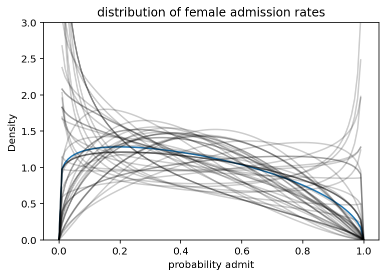
pbar = tf.reduce_mean(tf.sigmoid(sample_alpha[:, gid]))
theta = tf.reduce_mean(sample_theta)
plt.plot(x, tf.exp(tfd.Beta(pbar * theta, (1 - pbar) * theta).log_prob(x)))
plt.gca().set(ylabel="Density", xlabel="probability admit", ylim=(0, 3))

# draw 50 beta distributions sampled from posterior
for i in range(50):
    p = tf.sigmoid(sample_alpha[i, gid])
    theta = sample_theta[i]
    plt.plot(
        x, tf.exp(tfd.Beta(p * theta, (1 - p) * theta).log_prob(x)), "k", alpha=0.2
    )
plt.title("distribution of female admission rates")
plt.show()

../_images/12_monsters_and_mixtures_22_0.png

Code 12.5¶

# get samples given the posterior distribution
N = tf.cast(d.applications.values, dtype=tf.float32)
gid = d.gid.values

sample_pbar = tf.sigmoid(tf.squeeze(tf.gather(sample_alpha, gid, axis=-1)))

# need to reshape it to make it happy
st = tf.reshape(sample_theta, shape=(1000, 1))

# prepare the concentration vector
concentration1 = sample_pbar * st
concentration0 = (1 - sample_pbar) * st

concentration = tf.stack([concentration1, concentration0], axis=-1)

dist = tfd.DirichletMultinomial(total_count=N, concentration=concentration)

predictive_samples = dist.sample()

# numpy style indexing magic ! .. hate it !
admit_rate = predictive_samples[::, ::, 0] / N

plt.scatter(range(1, 13), d.admit.values / N)
plt.errorbar(
    range(1, 13),
    np.mean(admit_rate, 0),
    np.std(admit_rate, 0) / 2,
    fmt="o",
    c="k",
    mfc="none",
    ms=7,
    elinewidth=1,
)
plt.plot(range(1, 13), np.percentile(admit_rate, 5.5, 0), "k+")
plt.plot(range(1, 13), np.percentile(admit_rate, 94.5, 0), "k+")
plt.show()

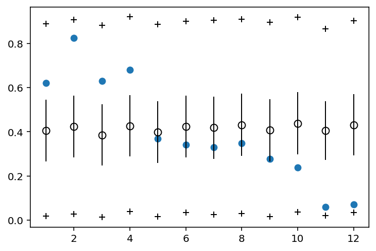
../_images/12_monsters_and_mixtures_26_0.png

In the above plot, the vertifical axis shows the predicted proportion admitted, for each case on the horizontal.

Blue points show the empirical proportion admitted on each row of data

Open circles are the posterior mean pbar and + symbols mark the 89% interval of predicted counts of admission

12.1.2 Negative-binomial or gamma-Poisson¶

Code 12.6 (Not working !)¶

Start to use Gamma-Poisson (also known as Negative Binomial) models.

Essentially Gamm-Poisson is about associating a rate to each Posisson count observation. Estimates the shape of gamma distribution to describe the Poisson rates across cases.

Gamma-Poisson also expects more variation around the mean rate.

The negative binomial distribution arises naturally from a probability experiment of performing a series of independent Bernoulli trials until the occurrence of the rth success where r is a positive integer.

d = RethinkingDataset.Kline.get_dataset()
d["P"] = d.population.pipe(np.log).pipe(lambda x: (x - x.mean()) / x.std())
d["cid"] = (d.contact == "high").astype(int)

d.head()

	culture	population	contact	total_tools	mean_TU	P	cid
0	Malekula	1100	low	13	3.2	-1.291473	0
1	Tikopia	1500	low	22	4.7	-1.088551	0
2	Santa Cruz	3600	low	24	4.0	-0.515765	0
3	Yap	4791	high	43	5.0	-0.328773	1
4	Lau Fiji	7400	high	33	5.0	-0.044339	1

def model_12_2(cid, P):
    def _generator():
        alpha = yield Root(tfd.Sample(tfd.Normal(loc=1.0, scale=1.0), sample_shape=2))
        beta = yield Root(tfd.Sample(tfd.Exponential(rate=1.0), sample_shape=2))
        gamma = yield Root(tfd.Sample(tfd.Exponential(rate=1.0), sample_shape=1))
        phi = yield Root(tfd.Sample(tfd.Exponential(rate=1.0), sample_shape=1))

        lambda_ = (
            tf.exp(tf.squeeze(tf.gather(alpha, cid, axis=-1)))
            * tf.math.pow(P, tf.squeeze(tf.gather(beta, cid, axis=-1)))
            / gamma
        )

        g_concentration = lambda_ / phi
        g_rate = 1 / phi

        t1 = yield tfd.Independent(
            tfd.Gamma(concentration=g_concentration, rate=g_rate),
            reinterpreted_batch_ndims=1,
        )

        T = yield tfd.Independent(tfd.Poisson(rate=t1), reinterpreted_batch_ndims=1)

    return tfd.JointDistributionCoroutine(_generator, validate_args=True)


jdc_12_2 = model_12_2(d.cid.values, tf.cast(d.P.values, dtype=tf.float32))

# Issue -
# Even prior sampling is not coming back !
# jdc_12_2.sample()

# NUMBER_OF_CHAINS_12_2 = 1

# alpha_init, beta_init, gamma_init, phi_init, t1_init, _ = jdc_12_2.sample(2)

# init_state = [
#     alpha_init,
#     beta_init,
#     gamma_init,
#     phi_init,
#     t1_init
# ]

# bijectors = [
#     tfb.Identity(),
#     tfb.Exp(),
#     tfb.Exp(),
#     tfb.Exp(),
#     tfb.Identity(),
# ]

# posterior_12_2, trace_12_2 = sample_posterior(jdc_12_2,
#                                    observed_data=(d.total_tools.values,),
#                                    init_state=init_state,
#                                    bijectors=bijectors,
#                                    params=['alpha', 'beta', 'gamma' 'phi', 't1'])

# az.summary(trace_12_2, credible_interval=0.89)

Statistical Rethinking (2nd Edition)

12. Monsters and Mixtures

Contents