.ipynb .pdf

repository open issue

Binder

Contents

11. God Spiked the Integers

# Install packages that are not installed in colab
try:
  import google.colab
  %pip install -q watermark
  %pip install git+https://github.com/ksachdeva/rethinking-tensorflow-probability.git
except:
  pass

%load_ext watermark

# Core
import numpy as np
import arviz as az
import pandas as pd
import xarray as xr
import tensorflow as tf
import tensorflow_probability as tfp

# visualization
import matplotlib.pyplot as plt

from rethinking.data import RethinkingDataset
from rethinking.data import dataframe_to_tensors
from rethinking.mcmc import sample_posterior

# aliases
tfd = tfp.distributions
tfb = tfp.bijectors
Root = tfd.JointDistributionCoroutine.Root

2022-01-19 19:12:08.073507: W tensorflow/stream_executor/platform/default/dso_loader.cc:64] Could not load dynamic library 'libcudart.so.11.0'; dlerror: libcudart.so.11.0: cannot open shared object file: No such file or directory
2022-01-19 19:12:08.073545: I tensorflow/stream_executor/cuda/cudart_stub.cc:29] Ignore above cudart dlerror if you do not have a GPU set up on your machine.

%watermark -p numpy,tensorflow,tensorflow_probability,arviz,scipy,pandas,rethinking

numpy                 : 1.21.5
tensorflow            : 2.7.0
tensorflow_probability: 0.15.0
arviz                 : 0.11.4
scipy                 : 1.7.3
pandas                : 1.3.5
rethinking            : 0.1.0

# config of various plotting libraries
%config InlineBackend.figure_format = 'retina'

11.1 Binomial regression

11.1.1 Logistic regression: Prosocial chimpanzees

Code 11.1

Authors start the chapter by highlighting one key difference between Generalized Linear Models and Gaussian Linear Models. He says, that unlike Gaussian Linear Models where we had some interpretation of parameters, in the case of GLM it is the combination of parameters that matter.

Most common & useful GLM models are about counts but they are also difficult to model. What is the reason for that ?

He says - “When we wish to predict the outcome in the form of counts, the scale of parameters is never the same as the scale of outcome. This is another way of saying that it is the combination of parameters that help in prediction and hence some where we lose human intution that could have connected the parmaeters with the outcome.

Binomial Regression -: model the outcome (count) when both of the categories are known.

Poisson Regression -: model the outcome (count) when the maximum count is unknown.

d = RethinkingDataset.Chimpanzees.get_dataset()

Code 11.2

We aim to build index variables instead of using dummy variables. Below is a quick way to do it. Treatment here is about the 4 possible situations.

1. prosoc_left= 0 and condition= 0: Two food items on right and no partner.

2. prosoc_left= 1 and condition= 0: Two food items on left and no partner.

3. prosoc_left= 0 and condition= 1: Two food items on right and partner present.

4. prosoc_left= 1 and condition= 1: Two food items on left and partner present.

# In the book there is an additional 1 in the code snippet.
# That is because of R as in R index does not starts with 0

d["treatment"] = d.prosoc_left + 2 * d.condition

Code 11.3

d.reset_index().groupby(["condition", "prosoc_left", "treatment"]).count()["index"]

condition  prosoc_left  treatment
0          0            0            126
           1            1            126
1          0            2            126
           1            3            126
Name: index, dtype: int64

d.describe()

	actor	recipient	condition	block	trial	prosoc_left	chose_prosoc	pulled_left	treatment
count	504.000000	252.00000	504.000000	504.000000	504.000000	504.000000	504.00000	504.000000	504.000000
mean	4.000000	5.00000	0.500000	3.500000	36.500000	0.500000	0.56746	0.579365	1.500000
std	2.001987	2.00398	0.500497	1.709522	20.803253	0.500497	0.49592	0.494151	1.119145
min	1.000000	2.00000	0.000000	1.000000	1.000000	0.000000	0.00000	0.000000	0.000000
25%	2.000000	3.00000	0.000000	2.000000	18.750000	0.000000	0.00000	0.000000	0.750000
50%	4.000000	5.00000	0.500000	3.500000	36.500000	0.500000	1.00000	1.000000	1.500000
75%	6.000000	7.00000	1.000000	5.000000	54.250000	1.000000	1.00000	1.000000	2.250000
max	7.000000	8.00000	1.000000	6.000000	72.000000	1.000000	1.00000	1.000000	3.000000

Code 11.4

def model_11_1(alpha_scale):
    def _generator():
        alpha = yield Root(
            tfd.Sample(tfd.Normal(loc=0.0, scale=alpha_scale), sample_shape=1)
        )
        logit = alpha
        pulled_left = yield tfd.Independent(
            tfd.Binomial(total_count=1.0, logits=logit), reinterpreted_batch_ndims=1
        )

    return tfd.JointDistributionCoroutine(_generator, validate_args=True)


jdc_11_1 = model_11_1(alpha_scale=10.0)

Code 11.5

prior = jdc_11_1.sample(1000)

2022-01-19 19:12:11.023338: W tensorflow/stream_executor/platform/default/dso_loader.cc:64] Could not load dynamic library 'libcuda.so.1'; dlerror: libcuda.so.1: cannot open shared object file: No such file or directory
2022-01-19 19:12:11.023377: W tensorflow/stream_executor/cuda/cuda_driver.cc:269] failed call to cuInit: UNKNOWN ERROR (303)
2022-01-19 19:12:11.023402: I tensorflow/stream_executor/cuda/cuda_diagnostics.cc:156] kernel driver does not appear to be running on this host (fv-az272-145): /proc/driver/nvidia/version does not exist
2022-01-19 19:12:11.023622: I tensorflow/core/platform/cpu_feature_guard.cc:151] This TensorFlow binary is optimized with oneAPI Deep Neural Network Library (oneDNN) to use the following CPU instructions in performance-critical operations:  AVX2 FMA
To enable them in other operations, rebuild TensorFlow with the appropriate compiler flags.

Code 11.6

p = tf.math.sigmoid(prior[0])
az.plot_kde(p.numpy())
plt.show()

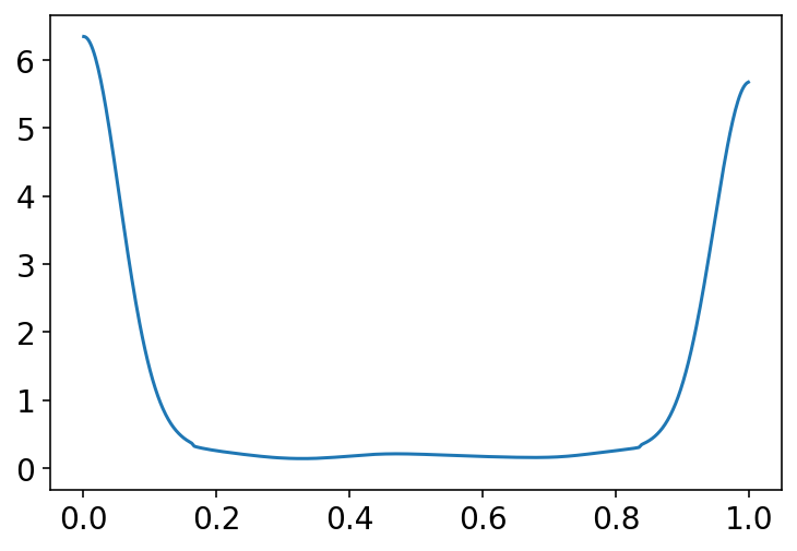
Most of the probability mass in the above plot is piled up near zero or one. A flat prior in the logit space is not a flat prior in the outcome probability space.

jdc_11_1b = model_11_1(alpha_scale=1.5)
prior_with_1_5 = jdc_11_1b.sample(1000)

p = tf.math.sigmoid(prior_with_1_5[0])

az.plot_kde(p.numpy())
plt.show()

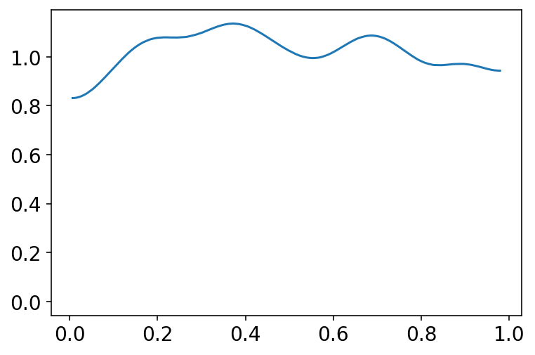
A more concentrated Normal(0,1.5) prior produces something more reasonable

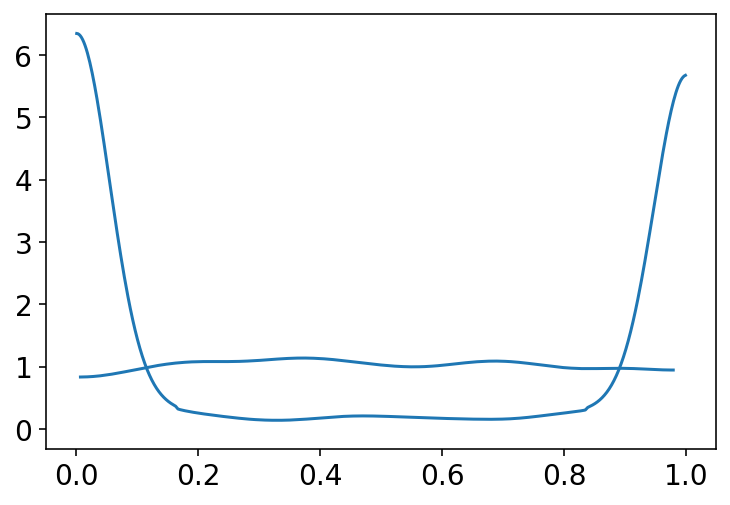
# simply showing both of the above plots
# at the same time to reproduce figure 11.3

p1 = tf.math.sigmoid(prior[0])
p2 = tf.math.sigmoid(prior_with_1_5[0])
az.plot_kde(p1.numpy())
az.plot_kde(p2.numpy())
plt.show()

Code 11.7

tdf = dataframe_to_tensors("Chimpanzee", d, {"treatment": tf.int32})

def model_11_2(treatments):
    def _generator():
        alpha = yield Root(tfd.Sample(tfd.Normal(loc=0.0, scale=1.5), sample_shape=1))
        beta_treatment = yield Root(
            tfd.Sample(tfd.Normal(loc=0.0, scale=10.0), sample_shape=4)
        )

        logit = alpha + tf.squeeze(tf.gather(beta_treatment, treatments, axis=-1))

        pulled_left = yield tfd.Independent(
            tfd.Binomial(total_count=1.0, logits=logit), reinterpreted_batch_ndims=1
        )

    return tfd.JointDistributionCoroutine(_generator, validate_args=False)


jdc_11_2 = model_11_2(tdf.treatment)

prior_a, prior_b, _ = jdc_11_2.sample(1000)

prior_a = prior_a.numpy()
prior_b = prior_b.numpy()

def compute_p_for_given_treatment(t):
    p = prior_a[:, 0] + prior_b[:, t]
    return tf.math.sigmoid(p)


p = np.array(list(map(compute_p_for_given_treatment, np.arange(4)))).T

p.shape

(1000, 4)

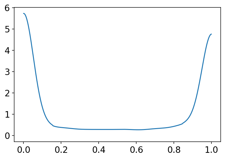
Code 11.8

az.plot_kde(np.abs(p[:, 0] - p[:, 1]))
plt.show()

Code 11.9

Sample model as 11_2 but with a different scale for beta_treatment

def model_11_3(treatments):
    def _generator():
        alpha = yield Root(tfd.Sample(tfd.Normal(loc=0.0, scale=1.5), sample_shape=1))
        beta_treatment = yield Root(
            tfd.Sample(tfd.Normal(loc=0.0, scale=0.5), sample_shape=4)
        )

        logit = alpha + tf.squeeze(tf.gather(beta_treatment, treatments, axis=-1))

        pulled_left = yield tfd.Independent(
            tfd.Binomial(total_count=1.0, logits=logit), reinterpreted_batch_ndims=1
        )

    return tfd.JointDistributionCoroutine(_generator, validate_args=False)


jdc_11_3 = model_11_3(tdf.treatment)


prior_a, prior_b, _ = jdc_11_3.sample(1000)

prior_a = prior_a.numpy()
prior_b = prior_b.numpy()

p = np.array(list(map(compute_p_for_given_treatment, np.arange(4)))).T

np.mean(np.abs(p[:, 0] - p[:, 1]))

0.096076064

Code 11.10

d

	actor	recipient	condition	block	trial	prosoc_left	chose_prosoc	pulled_left	treatment
0	1	NaN	0	1	2	0	1	0	0
1	1	NaN	0	1	4	0	0	1	0
2	1	NaN	0	1	6	1	0	0	1
3	1	NaN	0	1	8	0	1	0	0
4	1	NaN	0	1	10	1	1	1	1
...	...	...	...	...	...	...	...	...	...
499	7	4.0	1	6	64	1	1	1	3
500	7	6.0	1	6	66	1	1	1	3
501	7	3.0	1	6	68	0	0	1	2
502	7	7.0	1	6	70	0	0	1	2
503	7	2.0	1	6	72	0	0	1	2

504 rows × 9 columns

d["actor_id"] = d.actor.values - 1

tdf = dataframe_to_tensors(
    "Chimpanzee",
    d,
    {"pulled_left": tf.float32, "treatment": tf.int32, "actor_id": tf.int32},
)

Code 11.11

def model_11_4(actors, treatments):
    def _generator():
        alpha = yield Root(tfd.Sample(tfd.Normal(loc=0.0, scale=1.5), sample_shape=7))
        beta_treatment = yield Root(
            tfd.Sample(tfd.Normal(loc=0.0, scale=0.5), sample_shape=4)
        )

        term1 = tf.gather(alpha, actors, axis=-1)
        term2 = tf.gather(beta_treatment, treatments, axis=-1)

        logit = term1 + term2

        pulled_left = yield tfd.Independent(
            tfd.Binomial(total_count=1.0, logits=logit), reinterpreted_batch_ndims=1
        )

    return tfd.JointDistributionCoroutine(_generator, validate_args=False)


jdc_11_4 = model_11_4(tdf.actor_id, tdf.treatment)
jdc_11_4.sample()

StructTuple(
  var0=<tf.Tensor: shape=(7,), dtype=float32, numpy=
    array([ 0.72694427,  0.97887087, -0.77214324, -2.3240948 ,  0.29000178,
            0.5599559 ,  0.01908719], dtype=float32)>,
  var1=<tf.Tensor: shape=(4,), dtype=float32, numpy=array([ 0.16739044,  0.06596012, -0.5800672 , -0.34271017], dtype=float32)>,
  var2=<tf.Tensor: shape=(504,), dtype=float32, numpy=
    array([1., 0., 1., 1., 0., 0., 1., 1., 1., 0., 1., 0., 0., 1., 1., 1., 0.,
           0., 1., 1., 0., 1., 0., 1., 1., 1., 0., 0., 1., 1., 1., 1., 1., 1.,
           0., 1., 1., 1., 1., 1., 1., 1., 0., 1., 0., 1., 1., 0., 0., 1., 1.,
           1., 0., 1., 0., 1., 0., 0., 1., 0., 1., 1., 1., 1., 1., 1., 1., 1.,
           1., 1., 1., 1., 1., 1., 1., 0., 1., 1., 1., 0., 1., 1., 1., 0., 0.,
           1., 1., 1., 1., 1., 1., 1., 1., 1., 1., 0., 0., 1., 1., 0., 0., 1.,
           1., 1., 1., 1., 1., 1., 1., 1., 0., 1., 1., 1., 0., 1., 1., 0., 1.,
           0., 1., 1., 1., 1., 0., 1., 1., 0., 0., 1., 1., 1., 1., 1., 0., 0.,
           0., 1., 0., 1., 1., 0., 0., 0., 1., 0., 0., 0., 0., 1., 1., 0., 0.,
           0., 1., 0., 0., 0., 0., 0., 0., 0., 1., 0., 1., 0., 0., 0., 0., 1.,
           0., 0., 0., 1., 0., 0., 1., 0., 0., 1., 0., 1., 0., 0., 0., 0., 0.,
           0., 1., 0., 0., 1., 1., 1., 0., 0., 0., 0., 1., 0., 1., 0., 1., 0.,
           0., 0., 0., 0., 0., 0., 1., 0., 0., 0., 0., 0., 0., 0., 1., 0., 1.,
           0., 0., 0., 0., 0., 0., 0., 1., 0., 0., 0., 0., 0., 0., 0., 1., 0.,
           0., 1., 0., 0., 0., 0., 0., 0., 0., 0., 0., 0., 1., 0., 0., 0., 0.,
           0., 0., 0., 0., 0., 0., 0., 1., 0., 0., 0., 1., 0., 0., 0., 0., 0.,
           0., 0., 0., 1., 0., 0., 0., 0., 0., 0., 0., 0., 0., 0., 0., 0., 1.,
           1., 1., 1., 1., 1., 1., 0., 1., 1., 0., 1., 1., 1., 1., 0., 0., 0.,
           0., 1., 1., 1., 1., 0., 0., 0., 0., 1., 0., 0., 1., 0., 1., 1., 1.,
           1., 1., 0., 0., 0., 0., 1., 1., 0., 1., 1., 1., 1., 0., 1., 0., 0.,
           1., 1., 1., 0., 1., 0., 1., 0., 1., 0., 1., 1., 0., 1., 1., 0., 1.,
           1., 0., 0., 0., 1., 0., 0., 1., 1., 1., 1., 1., 1., 1., 1., 1., 0.,
           1., 1., 1., 1., 0., 0., 1., 1., 1., 0., 1., 1., 1., 0., 1., 1., 1.,
           1., 1., 0., 1., 1., 0., 0., 0., 1., 0., 0., 1., 0., 1., 0., 1., 0.,
           0., 1., 0., 1., 0., 0., 0., 0., 1., 0., 0., 1., 0., 1., 1., 0., 0.,
           1., 0., 1., 1., 0., 0., 0., 1., 1., 1., 1., 1., 0., 1., 1., 1., 1.,
           0., 0., 1., 1., 1., 1., 1., 1., 1., 1., 1., 0., 1., 1., 1., 0., 1.,
           1., 1., 0., 1., 1., 0., 0., 0., 0., 1., 0., 0., 0., 0., 0., 0., 0.,
           1., 0., 0., 1., 1., 0., 0., 1., 0., 1., 0., 0., 0., 0., 1., 1., 1.,
           1., 1., 0., 0., 1., 0., 0., 0., 0., 0., 0.], dtype=float32)>
)

NUMBER_OF_CHAINS = 2

init_state = [tf.zeros([NUMBER_OF_CHAINS, 7]), tf.zeros([NUMBER_OF_CHAINS, 4])]

bijectors = [tfb.Identity(), tfb.Identity()]

observed_data = (tdf.pulled_left,)

posterior_11_4, trace_11_4 = sample_posterior(
    jdc_11_4,
    observed_data=observed_data,
    init_state=init_state,
    bijectors=bijectors,
    params=["alpha", "beta_treatment"],
)


az.summary(trace_11_4, hdi_prob=0.89)

WARNING:tensorflow:@custom_gradient grad_fn has 'variables' in signature, but no ResourceVariables were used on the forward pass.

	mean	sd	hdi_5.5%	hdi_94.5%	mcse_mean	mcse_sd	ess_bulk	ess_tail	r_hat
alpha[0]	-0.420	0.332	-0.899	0.145	0.015	0.011	481.0	468.0	1.01
alpha[1]	3.872	0.720	2.693	4.921	0.041	0.030	320.0	334.0	1.00
alpha[2]	-0.726	0.338	-1.228	-0.186	0.015	0.010	533.0	406.0	1.02
alpha[3]	-0.731	0.331	-1.253	-0.214	0.014	0.010	543.0	545.0	1.01
alpha[4]	-0.431	0.332	-0.886	0.208	0.014	0.010	537.0	523.0	1.00
alpha[5]	0.502	0.337	-0.065	1.002	0.015	0.011	485.0	524.0	1.00
alpha[6]	1.972	0.431	1.292	2.636	0.018	0.014	649.0	201.0	1.02
beta_treatment[0]	-0.060	0.275	-0.485	0.389	0.020	0.014	197.0	372.0	1.03
beta_treatment[1]	0.455	0.290	-0.062	0.843	0.018	0.013	270.0	362.0	1.02
beta_treatment[2]	-0.370	0.282	-0.886	0.007	0.016	0.012	297.0	417.0	1.01
beta_treatment[3]	0.353	0.293	-0.158	0.778	0.018	0.013	278.0	481.0	1.01

Clearly interpretation of all these varying parameters is difficult now. The alphas above represent intercepts unique to each chimpanzee. Each of these expresses the tendency of each individual to pull the left lever.

Code 11.12

post = trace_11_4.posterior
p_left = tf.math.sigmoid(post["alpha"].values)
az.plot_forest({"p_left": p_left}, combined=True, hdi_prob=0.89)
plt.gca().set(xlim=(-0.01, 1.01))
plt.show()

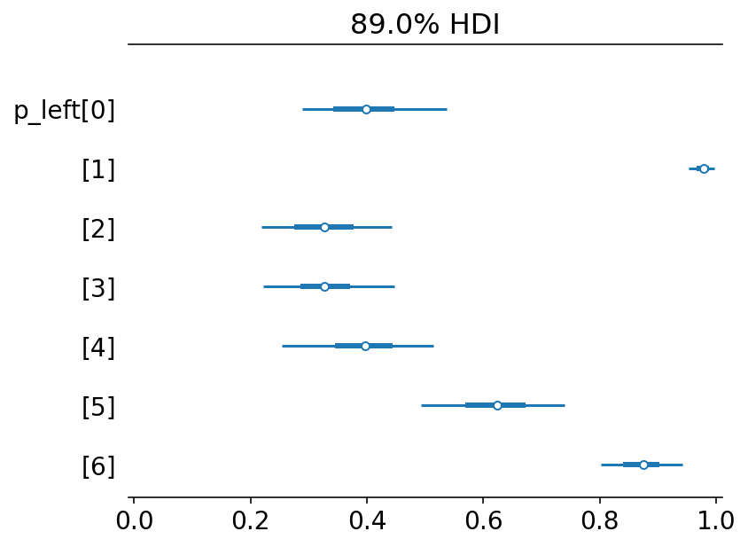
What above plot shows is that 0,2,3,4 show preference for right lever. Two chimps (1 & 6) show strong preference for left lever and it is also reflected in the data

Code 11.13

Here we are now considering treatment effects and hoping that they are estimated more precisely

labs = ["R/N", "L/N", "R/P", "L/P"]
az.plot_forest(trace_11_4, combined=True, var_names="beta_treatment", hdi_prob=0.89)
plt.gca().set_yticklabels(labs[::-1])
plt.show()

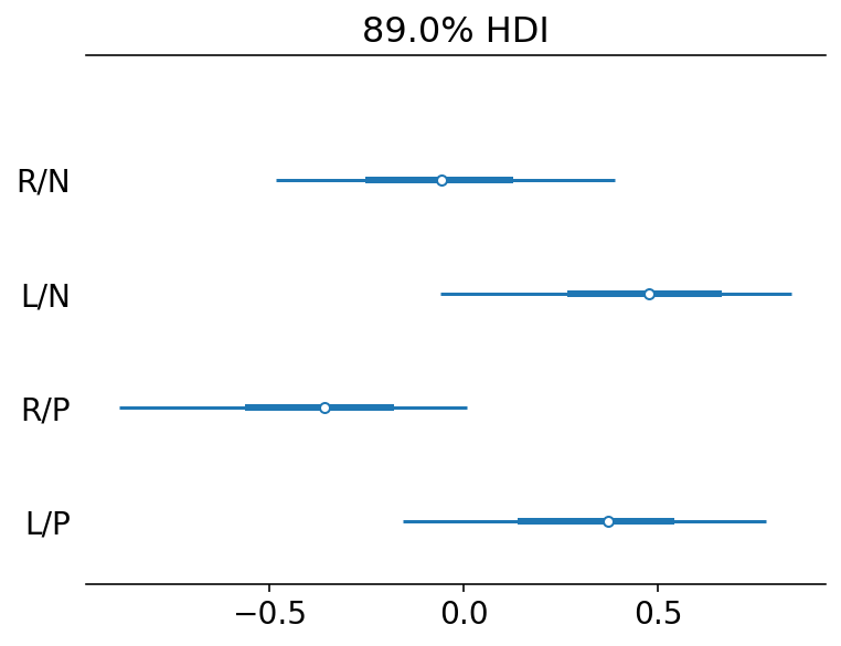
• L/N => prosocial on left / no partner

• R/P => proscoial on right / partner

What we are looking for is evidence that the chimpanzees choose the prosocial option more when a partner is present. This implies comparing the first row with the third row and the second row with the fourth row

Code 11.14

diffs = {
    "db13": post["beta_treatment"][..., 0] - post["beta_treatment"][..., 2],
    "db24": post["beta_treatment"][..., 1] - post["beta_treatment"][..., 3],
}
az.plot_forest(diffs, combined=True)
plt.show()

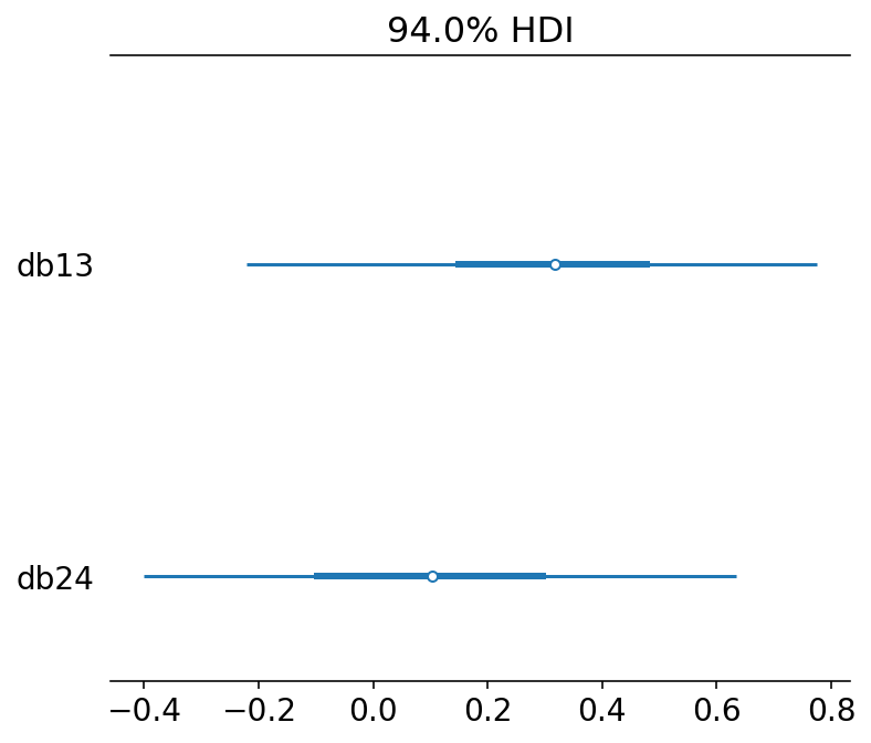
db13 is the difference between no-partner/partner treatments when the prosocial option was on the right.

There is a weak evidence that individual pulled left more when the partner was absent

Code 11.15

Compute proportion in each combination of actor & treatment

pl = d.groupby(["actor", "treatment"])["pulled_left"].mean().unstack()
pl.iloc[0, :]

treatment
0    0.333333
1    0.500000
2    0.277778
3    0.555556
Name: 1, dtype: float64

pl

treatment	0	1	2	3
actor
1	0.333333	0.500000	0.277778	0.555556
2	1.000000	1.000000	1.000000	1.000000
3	0.277778	0.611111	0.166667	0.333333
4	0.333333	0.500000	0.111111	0.444444
5	0.333333	0.555556	0.277778	0.500000
6	0.777778	0.611111	0.555556	0.611111
7	0.777778	0.833333	0.944444	1.000000

the cells contain proportions of pulls that were of the left lever

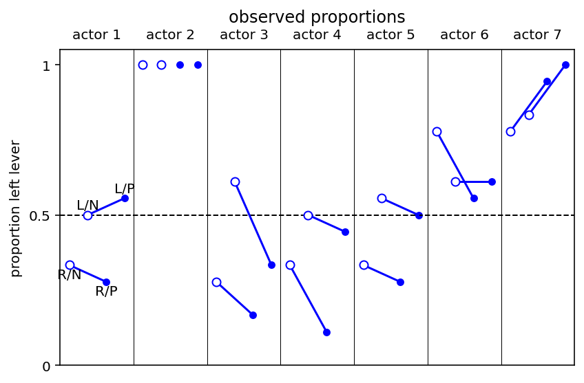
Code 11.16

Plotting observed proportions

ax = plt.subplot(
    xlim=(0.5, 28.5),
    ylim=(0, 1.05),
    xlabel="",
    ylabel="proportion left lever",
    xticks=[],
)
plt.yticks(ticks=[0, 0.5, 1], labels=[0, 0.5, 1])
ax.axhline(0.5, c="k", lw=1, ls="--")
for j in range(1, 8):
    ax.axvline((j - 1) * 4 + 4.5, c="k", lw=0.5)
for j in range(1, 8):
    ax.annotate(
        "actor {}".format(j),
        ((j - 1) * 4 + 2.5, 1.1),
        ha="center",
        va="center",
        annotation_clip=False,
    )
for j in np.delete(range(1, 8), 1):
    ax.plot((j - 1) * 4 + np.array([1, 3]), pl.loc[j, [0, 2]], "b")
    ax.plot((j - 1) * 4 + np.array([2, 4]), pl.loc[j, [1, 3]], "b")
x = np.arange(1, 29).reshape(7, 4)
ax.scatter(
    x[:, [0, 1]].reshape(-1),
    pl.values[:, [0, 1]].reshape(-1),
    edgecolor="b",
    facecolor="w",
    zorder=3,
)
ax.scatter(
    x[:, [2, 3]].reshape(-1), pl.values[:, [2, 3]].reshape(-1), marker=".", c="b", s=80
)
yoff = 0.01
ax.annotate("R/N", (1, pl.loc[1, 0] - yoff), ha="center", va="top")
ax.annotate("L/N", (2, pl.loc[1, 1] + yoff), ha="center", va="bottom")
ax.annotate("R/P", (3, pl.loc[1, 2] - yoff), ha="center", va="top")
ax.annotate("L/P", (4, pl.loc[1, 3] + yoff), ha="center", va="bottom")
ax.set_title("observed proportions\n")
plt.tight_layout()

Code 11.17

dat = {"actor": np.repeat(np.arange(7), 4), "treatment": np.tile(np.arange(4), 7)}


def compute_p_for_given_actor_treatment(params):
    a = params[0]
    t = params[1]
    p = post["alpha"].values[0][:, a] + post["beta_treatment"].values[0][:, t]
    return tf.math.sigmoid(p)


params = zip(dat["actor"], dat["treatment"])

p = np.array(list(map(compute_p_for_given_actor_treatment, params))).T

p_mu = np.mean(p, 0)
p_ci = np.percentile(p, q=(4.5, 95.5), axis=0)

Code 11.18

d["side"] = d.prosoc_left  # right 0, left 1
d["cond"] = d.condition  # no partner 0, partner 1

Code 11.19

tdf = dataframe_to_tensors(
    "Chimpanzee",
    d,
    {
        "pulled_left": tf.float32,
        "actor_id": tf.int32,
        "side": tf.int32,
        "cond": tf.int32,
    },
)


def model_11_5(actors, sides, conds):
    def _generator():
        alpha = yield Root(tfd.Sample(tfd.Normal(loc=0.0, scale=1.5), sample_shape=7))
        beta_side = yield Root(
            tfd.Sample(tfd.Normal(loc=0.0, scale=0.5), sample_shape=2)
        )
        beta_cond = yield Root(
            tfd.Sample(tfd.Normal(loc=0.0, scale=0.5), sample_shape=2)
        )

        term1 = tf.gather(alpha, actors, axis=-1)
        term2 = tf.gather(beta_side, sides, axis=-1)
        term3 = tf.gather(beta_cond, conds, axis=-1)

        logit = term1 + term2 + term3

        pulled_left = yield tfd.Independent(
            tfd.Binomial(total_count=1.0, logits=logit), reinterpreted_batch_ndims=1
        )

    return tfd.JointDistributionCoroutine(_generator, validate_args=False)


jdc_11_5 = model_11_5(tdf.actor_id, tdf.side, tdf.cond)
jdc_11_5.sample()

StructTuple(
  var0=<tf.Tensor: shape=(7,), dtype=float32, numpy=
    array([-1.5783112 ,  0.5358548 , -2.0334883 ,  0.93882376,  0.03772911,
           -1.7945005 ,  1.2174203 ], dtype=float32)>,
  var1=<tf.Tensor: shape=(2,), dtype=float32, numpy=array([ 0.24999732, -0.52624685], dtype=float32)>,
  var2=<tf.Tensor: shape=(2,), dtype=float32, numpy=array([0.7743274 , 0.52075315], dtype=float32)>,
  var3=<tf.Tensor: shape=(504,), dtype=float32, numpy=
    array([0., 1., 1., 0., 1., 0., 1., 0., 1., 1., 0., 0., 0., 0., 1., 0., 0.,
           1., 0., 0., 0., 0., 0., 1., 0., 0., 0., 1., 1., 0., 0., 1., 0., 0.,
           1., 0., 0., 1., 0., 0., 1., 1., 1., 1., 0., 1., 0., 1., 0., 1., 0.,
           0., 0., 0., 0., 0., 0., 0., 0., 1., 0., 0., 0., 0., 0., 0., 0., 0.,
           0., 0., 1., 0., 1., 1., 1., 1., 1., 1., 1., 1., 0., 1., 0., 1., 1.,
           0., 1., 0., 1., 1., 1., 1., 1., 1., 0., 1., 1., 1., 0., 0., 0., 1.,
           1., 1., 1., 1., 1., 1., 1., 1., 0., 1., 1., 1., 1., 1., 1., 1., 1.,
           1., 0., 1., 0., 1., 1., 1., 0., 1., 1., 1., 1., 1., 0., 1., 1., 1.,
           0., 1., 1., 1., 1., 0., 1., 1., 0., 0., 0., 0., 0., 0., 0., 1., 0.,
           0., 0., 0., 0., 1., 0., 0., 0., 0., 0., 1., 0., 0., 1., 0., 1., 0.,
           0., 1., 0., 0., 0., 1., 0., 0., 1., 0., 0., 0., 0., 0., 0., 1., 0.,
           0., 1., 1., 0., 0., 0., 0., 0., 0., 0., 1., 0., 0., 0., 0., 0., 0.,
           0., 0., 1., 0., 0., 0., 1., 0., 1., 0., 0., 0., 1., 1., 0., 1., 1.,
           1., 1., 1., 1., 1., 1., 1., 1., 0., 1., 1., 1., 1., 1., 0., 1., 1.,
           1., 1., 1., 1., 1., 1., 0., 1., 1., 1., 1., 1., 1., 1., 1., 1., 1.,
           1., 1., 1., 1., 0., 0., 1., 1., 1., 1., 1., 0., 1., 1., 1., 0., 1.,
           1., 1., 1., 1., 0., 1., 1., 0., 1., 1., 1., 1., 1., 1., 1., 0., 0.,
           1., 1., 1., 0., 0., 1., 1., 1., 0., 1., 1., 0., 1., 0., 1., 0., 1.,
           1., 1., 0., 1., 1., 1., 0., 1., 0., 1., 1., 1., 0., 1., 0., 1., 1.,
           1., 1., 0., 1., 1., 1., 0., 1., 0., 0., 0., 1., 1., 1., 0., 0., 1.,
           1., 0., 1., 0., 1., 1., 1., 0., 1., 1., 1., 0., 1., 1., 1., 1., 1.,
           1., 0., 0., 1., 0., 0., 0., 0., 0., 0., 0., 0., 0., 0., 0., 1., 0.,
           0., 0., 0., 0., 1., 0., 0., 0., 0., 0., 0., 0., 1., 0., 1., 0., 0.,
           0., 1., 0., 0., 0., 0., 0., 1., 0., 0., 1., 0., 0., 0., 0., 0., 0.,
           0., 0., 0., 0., 1., 0., 0., 1., 1., 0., 0., 1., 0., 0., 0., 0., 0.,
           0., 0., 1., 0., 0., 0., 0., 1., 1., 1., 0., 0., 1., 1., 1., 1., 1.,
           1., 1., 1., 0., 1., 1., 1., 1., 1., 1., 0., 1., 1., 1., 1., 1., 1.,
           1., 0., 1., 0., 1., 1., 0., 1., 1., 1., 1., 0., 1., 1., 1., 1., 1.,
           1., 1., 1., 0., 0., 1., 1., 1., 1., 1., 1., 1., 1., 1., 1., 0., 1.,
           0., 1., 1., 1., 1., 1., 1., 1., 1., 1., 1.], dtype=float32)>
)

init_state = [
    tf.zeros([NUMBER_OF_CHAINS, 7]),
    tf.zeros([NUMBER_OF_CHAINS, 2]),
    tf.zeros([NUMBER_OF_CHAINS, 2]),
]

bijectors = [tfb.Identity(), tfb.Identity(), tfb.Identity()]

observed_data = (tdf.pulled_left,)

posterior_11_5, trace_11_5 = sample_posterior(
    jdc_11_5,
    observed_data=observed_data,
    init_state=init_state,
    bijectors=bijectors,
    params=["alpha", "beta_side", "beta_cond"],
)


az.summary(trace_11_5, hdi_prob=0.89)

	mean	sd	hdi_5.5%	hdi_94.5%	mcse_mean	mcse_sd	ess_bulk	ess_tail	r_hat
alpha[0]	-0.702	0.424	-1.441	-0.098	0.040	0.028	114.0	144.0	1.00
alpha[1]	3.730	0.696	2.645	4.776	0.060	0.043	136.0	138.0	1.01
alpha[2]	-0.992	0.425	-1.709	-0.334	0.041	0.029	110.0	97.0	1.00
alpha[3]	-1.000	0.422	-1.593	-0.267	0.040	0.029	110.0	147.0	1.00
alpha[4]	-0.702	0.407	-1.339	-0.085	0.039	0.028	110.0	152.0	1.01
alpha[5]	0.220	0.419	-0.370	0.939	0.039	0.028	117.0	236.0	1.00
alpha[6]	1.699	0.462	1.026	2.480	0.039	0.028	142.0	229.0	1.00
beta_side[0]	-0.172	0.299	-0.584	0.346	0.019	0.013	250.0	468.0	1.00
beta_side[1]	0.525	0.317	0.049	1.045	0.022	0.016	203.0	146.0	1.00
beta_cond[0]	0.310	0.328	-0.267	0.785	0.025	0.018	168.0	360.0	1.01
beta_cond[1]	0.078	0.325	-0.478	0.550	0.025	0.018	171.0	337.0	1.00

Code 11.20

We need to compute likelihoods in order to use arviz’s compare method

def compute_and_store_log_likelihood_for_model_11_4():

    sample_alpha = posterior_11_4["alpha"]
    sample_beta = posterior_11_4["beta_treatment"]

    ds, _ = jdc_11_4.sample_distributions(value=[sample_alpha, sample_beta, None])

    log_likelihood_11_4 = ds[-1].distribution.log_prob(tdf.pulled_left).numpy()

    # we need to insert this in the sampler_stats
    sample_stats_11_4 = trace_11_4.sample_stats

    coords = [
        sample_stats_11_4.coords["chain"],
        sample_stats_11_4.coords["draw"],
        np.arange(504),
    ]

    sample_stats_11_4["log_likelihood"] = xr.DataArray(
        log_likelihood_11_4,
        coords=coords,
        dims=["chain", "draw", "log_likelihood_dim_0"],
    )


compute_and_store_log_likelihood_for_model_11_4()

def compute_and_store_log_likelihood_for_model_11_5():

    sample_alpha = posterior_11_5["alpha"]
    sample_beta_side = posterior_11_5["beta_side"]
    sample_beta_cond = posterior_11_5["beta_cond"]

    ds, _ = jdc_11_5.sample_distributions(
        value=[sample_alpha, sample_beta_side, sample_beta_cond, None]
    )

    log_likelihood_11_5 = ds[-1].distribution.log_prob(tdf.pulled_left).numpy()

    # we need to insert this in the sampler_stats
    sample_stats_11_5 = trace_11_5.sample_stats

    coords = [
        sample_stats_11_5.coords["chain"],
        sample_stats_11_5.coords["draw"],
        np.arange(504),
    ]

    sample_stats_11_5["log_likelihood"] = xr.DataArray(
        log_likelihood_11_5,
        coords=coords,
        dims=["chain", "draw", "log_likelihood_dim_0"],
    )


compute_and_store_log_likelihood_for_model_11_5()

az.compare({"m11.5": trace_11_5, "m11.4": trace_11_4}, ic="loo")

	rank	loo	p_loo	d_loo	weight	se	dse	warning	loo_scale
m11.5	0	-265.421100	7.883432	0.000000	1.0	9.528981	0.000000	False	log
m11.4	1	-266.360266	8.594999	0.939166	0.0	9.422382	0.675961	False	log

Overthinking: Adding log-probability calculations

Code 11.21

Since I am making use of xarray and above computation of likelihood has stored it as part of sample_stats here is one way to see it

trace_11_4.sample_stats

<xarray.Dataset>
Dimensions:               (chain: 2, draw: 500, log_likelihood_dim_0: 504)
Coordinates:
  * chain                 (chain) int64 0 1
  * draw                  (draw) int64 0 1 2 3 4 5 6 ... 494 495 496 497 498 499
  * log_likelihood_dim_0  (log_likelihood_dim_0) int64 0 1 2 3 ... 501 502 503
Data variables:
    mean_tree_accept      (chain, draw) float32 -0.1076 -3.67 ... 0.5353 0.08826
    log_likelihood        (chain, draw, log_likelihood_dim_0) float32 -0.4969...
Attributes:
    created_at:     2022-01-19T19:12:18.047055
    arviz_version:  0.11.4

xarray.Dataset

• Dimensions:
  • chain: 2
  • draw: 500
  • log_likelihood_dim_0: 504
• Coordinates: (3)
  • chain
    (chain)
    int64
    0 1

    array([0, 1])

  • draw
    (draw)
    int64
    0 1 2 3 4 5 ... 495 496 497 498 499

    array([  0,   1,   2, ..., 497, 498, 499])

  • log_likelihood_dim_0
    (log_likelihood_dim_0)
    int64
    0 1 2 3 4 5 ... 499 500 501 502 503

    array([  0,   1,   2, ..., 501, 502, 503])

• Data variables: (2)
  • mean_tree_accept
    (chain, draw)
    float32
    -0.1076 -3.67 ... 0.5353 0.08826

    array([[-1.07574463e-01, -3.67007446e+00, -5.21606445e-01,
            -2.99865723e-01, -2.74554443e+00, -1.12496948e+00,
            -5.53710938e-01, -1.91040039e-01,  2.01324463e-01,
            -1.56625366e+00, -3.46801758e-01,  1.46606445e-01,
            -1.75354004e+00, -1.60711670e+00, -3.29315186e-01,
            -1.39373779e-01, -1.58813477e-01, -3.37371826e-01,
             4.35272217e-01,  1.12182617e-01,  1.01226807e-01,
            -2.28881836e-01, -9.98535156e-02, -1.72155762e+00,
             4.71923828e-01, -3.89739990e-01, -7.26104736e-01,
            -3.97949219e-01,  3.05480957e-02, -7.13226318e-01,
            -7.47375488e-01, -4.60174561e-01,  1.41293335e+00,
            -8.40911865e-01,  1.77001953e-01, -1.06423950e+00,
             1.39569092e+00, -1.48864746e+00, -2.99682617e-01,
             1.40338135e+00, -1.96502686e+00, -1.36328125e+00,
            -2.72198486e+00, -4.44549561e-01, -1.17233276e+00,
            -1.23379517e+00,  4.65698242e-01, -5.16723633e-01,
            -9.87243652e-02, -3.75579834e-01, -2.25128174e-01,
            -6.23443604e-01, -1.69592285e+00, -2.90771484e-01,
             1.51025391e+00, -1.38580322e-01, -5.30364990e-01,
             8.84338379e-01, -3.32397461e-01, -8.59497070e-01,
    ...
            -1.47247314e+00, -2.57147217e+00,  9.13696289e-02,
            -4.84558105e-01,  4.05700684e-01,  2.01385498e-01,
            -9.16046143e-01,  1.20315552e+00, -3.56109619e-01,
            -4.10766602e-01, -2.42828369e+00, -3.02529907e+00,
            -7.60131836e-01, -5.57281494e-01,  9.35699463e-01,
             7.69104004e-01, -2.67333984e-01, -4.34844971e-01,
            -1.46597290e+00, -1.71786499e+00, -1.33276367e+00,
            -3.20343018e-01, -1.34457397e+00,  5.02441406e-01,
             6.33453369e-01,  7.29370117e-02, -3.94134521e-01,
            -2.99835205e-01,  1.14230347e+00, -7.42980957e-01,
            -3.22296143e-01,  7.34558105e-01, -8.02215576e-01,
            -6.86096191e-01, -1.27899170e-01, -1.13455200e+00,
            -2.16247559e-01, -7.73895264e-01,  2.12655640e+00,
            -4.80957031e-02,  6.65740967e-01, -1.24862671e+00,
            -1.63241577e+00, -6.90704346e-01, -1.44070435e+00,
             1.62600708e+00,  1.52191162e-01, -2.69500732e+00,
            -6.58142090e-01, -1.72210693e-01, -7.25891113e-01,
            -2.74505615e-01,  4.04418945e-01, -6.18774414e-01,
            -1.63787842e-01, -3.79150391e-01,  2.07946777e-01,
             5.35308838e-01,  8.82568359e-02]], dtype=float32)

  • log_likelihood
    (chain, draw, log_likelihood_dim_0)
    float32
    -0.4969 -0.9376 ... -0.1719 -0.1719

    array([[[-0.49688533, -0.9375725 , -0.659265  , ..., -0.19512506,
             -0.19512506, -0.19512506],
            [-0.49688533, -0.9375725 , -0.659265  , ..., -0.19512506,
             -0.19512506, -0.19512506],
            [-0.49688533, -0.9375725 , -0.659265  , ..., -0.19512506,
             -0.19512506, -0.19512506],
            ...,
            [-0.45679173, -1.0032445 , -0.64160895, ..., -0.17517945,
             -0.17517945, -0.17517945],
            [-0.40931696, -1.0909528 , -0.7799351 , ..., -0.2221993 ,
             -0.2221993 , -0.2221993 ],
            [-0.38085753, -1.1497221 , -0.7551726 , ..., -0.17337106,
             -0.17337106, -0.17337106]],
    
           [[-0.3778131 , -1.1563215 , -0.69897527, ..., -0.107118  ,
             -0.107118  , -0.107118  ],
            [-0.3778131 , -1.1563215 , -0.69897527, ..., -0.107118  ,
             -0.107118  , -0.107118  ],
            [-0.55311596, -0.8560305 , -0.73978204, ..., -0.38108376,
             -0.38108376, -0.38108376],
            ...,
            [-0.80237484, -0.594684  , -0.9990216 , ..., -0.17505877,
             -0.17505877, -0.17505877],
            [-0.4055789 , -1.0983846 , -0.616798  , ..., -0.1312735 ,
             -0.1312735 , -0.1312735 ],
            [-0.5539052 , -0.85496306, -0.9481497 , ..., -0.17193724,
             -0.17193724, -0.17193724]]], dtype=float32)

• Attributes: (2)

  created_at :

  2022-01-19T19:12:18.047055

  arviz_version :

  0.11.4

Code 11.22

This code cell in the book is showing how underneath Stan is computing the log likelihood and since I have been doing it anyways there is no need to fill this section.

See compute_and_store_log_likelihood_for_model_11_4 for the equivalent code

# nothing to do here

11.1.2 Relative shark and absolute penguin

Code 11.23

post = trace_11_4.posterior

np.mean(np.exp(post["beta_treatment"][:, :, 3] - post["beta_treatment"][:, :, 1]))

<xarray.DataArray 'beta_treatment' ()>
array(0.94151527, dtype=float32)

xarray.DataArray

'beta_treatment'

• 0.9415

  array(0.94151527, dtype=float32)

• Coordinates: (0)
• Attributes: (0)

Aggregated binomial: Chimpanzees again,condensed

Code 11.24

d = RethinkingDataset.Chimpanzees.get_dataset()
d["treatment"] = d.prosoc_left + 2 * d.condition
d["side"] = d.prosoc_left  # right 0, left 1
d["cond"] = d.condition  # no partner 0, partner 1
d_aggregated = (
    d.groupby(["treatment", "actor", "side", "cond"])["pulled_left"].sum().reset_index()
)
d_aggregated.rename(columns={"pulled_left": "left_pulls"}, inplace=True)

d_aggregated["actor_id"] = d_aggregated["actor"].values - 1

d_aggregated

	treatment	actor	side	cond	left_pulls	actor_id
0	0	1	0	0	6	0
1	0	2	0	0	18	1
2	0	3	0	0	5	2
3	0	4	0	0	6	3
4	0	5	0	0	6	4
5	0	6	0	0	14	5
6	0	7	0	0	14	6
7	1	1	1	0	9	0
8	1	2	1	0	18	1
9	1	3	1	0	11	2
10	1	4	1	0	9	3
11	1	5	1	0	10	4
12	1	6	1	0	11	5
13	1	7	1	0	15	6
14	2	1	0	1	5	0
15	2	2	0	1	18	1
16	2	3	0	1	3	2
17	2	4	0	1	2	3
18	2	5	0	1	5	4
19	2	6	0	1	10	5
20	2	7	0	1	17	6
21	3	1	1	1	10	0
22	3	2	1	1	18	1
23	3	3	1	1	6	2
24	3	4	1	1	8	3
25	3	5	1	1	9	4
26	3	6	1	1	11	5
27	3	7	1	1	18	6

Code 11.25

tdf = dataframe_to_tensors(
    "Chimpanzee",
    d_aggregated,
    {"actor_id": tf.int32, "treatment": tf.int32, "left_pulls": tf.float32},
)


def model_11_6(actors, treatments):
    def _generator():
        alpha = yield Root(tfd.Sample(tfd.Normal(loc=0.0, scale=1.5), sample_shape=7))
        beta_treatment = yield Root(
            tfd.Sample(tfd.Normal(loc=0.0, scale=0.5), sample_shape=4)
        )

        term1 = tf.gather(alpha, actors, axis=-1)
        term2 = tf.gather(beta_treatment, treatments, axis=-1)

        logit = term1 + term2

        pulled_left = yield tfd.Independent(
            tfd.Binomial(total_count=18.0, logits=logit), reinterpreted_batch_ndims=1
        )

    return tfd.JointDistributionCoroutine(_generator, validate_args=False)


jdc_11_6 = model_11_6(tdf.actor_id, tdf.treatment)
jdc_11_6.sample()

StructTuple(
  var0=<tf.Tensor: shape=(7,), dtype=float32, numpy=
    array([-0.7566206 ,  0.36602026,  1.1799304 , -2.2945683 ,  1.754464  ,
            1.5971856 , -0.06230567], dtype=float32)>,
  var1=<tf.Tensor: shape=(4,), dtype=float32, numpy=array([ 0.4967591 , -0.46505028, -0.63481325, -0.15960528], dtype=float32)>,
  var2=<tf.Tensor: shape=(28,), dtype=float32, numpy=
    array([ 7., 13., 16.,  3., 17., 13.,  9.,  3., 10.,  8.,  1., 13., 14.,
            5.,  6.,  7., 12.,  0., 16., 13.,  7.,  7., 10., 14.,  0., 17.,
           14., 11.], dtype=float32)>
)

init_state = [tf.zeros([NUMBER_OF_CHAINS, 7]), tf.zeros([NUMBER_OF_CHAINS, 4])]

bijectors = [tfb.Identity(), tfb.Identity()]

observed_data = (tdf.left_pulls,)

posterior_11_6, trace_11_6 = sample_posterior(
    jdc_11_6,
    observed_data=observed_data,
    init_state=init_state,
    bijectors=bijectors,
    params=["alpha", "beta_treatment"],
)


az.summary(trace_11_6, hdi_prob=0.89)

WARNING:tensorflow:@custom_gradient grad_fn has 'variables' in signature, but no ResourceVariables were used on the forward pass.

	mean	sd	hdi_5.5%	hdi_94.5%	mcse_mean	mcse_sd	ess_bulk	ess_tail	r_hat
alpha[0]	-0.456	0.337	-0.992	0.051	0.017	0.012	396.0	419.0	1.00
alpha[1]	3.828	0.739	2.696	4.916	0.041	0.029	327.0	383.0	1.00
alpha[2]	-0.741	0.334	-1.276	-0.233	0.016	0.011	457.0	312.0	1.00
alpha[3]	-0.759	0.358	-1.316	-0.179	0.016	0.012	488.0	343.0	1.00
alpha[4]	-0.459	0.325	-0.985	0.035	0.016	0.012	397.0	399.0	1.00
alpha[5]	0.486	0.346	-0.067	1.009	0.016	0.012	479.0	386.0	1.00
alpha[6]	1.936	0.356	1.318	2.441	0.017	0.012	444.0	334.0	1.00
beta_treatment[0]	-0.048	0.287	-0.513	0.400	0.016	0.011	334.0	326.0	1.00
beta_treatment[1]	0.476	0.282	0.033	0.929	0.017	0.012	261.0	352.0	1.00
beta_treatment[2]	-0.358	0.295	-0.811	0.115	0.017	0.012	287.0	274.0	1.01
beta_treatment[3]	0.372	0.292	-0.103	0.825	0.018	0.013	268.0	326.0	1.00

Code 11.26 (Find a way to get the comparison even if different number of obs)

# need to compute likelihood in order to do comparison


def compute_and_store_log_likelihood_for_model_11_6():

    sample_alpha = posterior_11_6["alpha"]
    sample_beta = posterior_11_6["beta_treatment"]

    ds, _ = jdc_11_6.sample_distributions(value=[sample_alpha, sample_beta, None])

    log_likelihood_11_6 = ds[-1].distribution.log_prob(tdf.left_pulls).numpy()

    # we need to insert this in the sampler_stats
    sample_stats_11_6 = trace_11_6.sample_stats

    coords = [
        sample_stats_11_6.coords["chain"],
        sample_stats_11_6.coords["draw"],
        np.arange(28),
    ]

    sample_stats_11_6["log_likelihood"] = xr.DataArray(
        log_likelihood_11_6,
        coords=coords,
        dims=["chain", "draw", "log_likelihood_dim_0"],
    )


compute_and_store_log_likelihood_for_model_11_6()

# in order to use comparison the number of observations should be same
# which is not the case with m11.4 (504) and m11.6 (28)
# and hence not able to compare using the arviz method

import warnings

try:
    az.compare({"m11.6": trace_11_6, "m11.4": trace_11_4}, ic="loo")
except Exception as e:
    warnings.warn("\n{}: {}".format(type(e).__name__, e))

/opt/hostedtoolcache/Python/3.7.12/x64/lib/python3.7/site-packages/arviz/stats/stats.py:695: UserWarning: Estimated shape parameter of Pareto distribution is greater than 0.7 for one or more samples. You should consider using a more robust model, this is because importance sampling is less likely to work well if the marginal posterior and LOO posterior are very different. This is more likely to happen with a non-robust model and highly influential observations.
  "Estimated shape parameter of Pareto distribution is greater than 0.7 for "

/opt/hostedtoolcache/Python/3.7.12/x64/lib/python3.7/site-packages/ipykernel_launcher.py:10: UserWarning: 
ValueError: The number of observations should be the same across all models
  # Remove the CWD from sys.path while we load stuff.

Code 11.27

# deviance of aggregated 6-in-9
print(-2 * tfd.Binomial(total_count=9.0, probs=0.2).log_prob(6))
# deviance of dis-aggregated
print(
    -2
    * np.sum(tfd.Bernoulli(probs=0.2).log_prob(np.array([1, 1, 1, 1, 1, 1, 0, 0, 0])))
)

WARNING:tensorflow:@custom_gradient grad_fn has 'variables' in signature, but no ResourceVariables were used on the forward pass.

tf.Tensor(11.7904825, shape=(), dtype=float32)
20.652116775512695

11.1.4 Aggregated binomial: Graduate school admissions

Code 11.28

Evaluate if there is a gender bias in admissions

d = RethinkingDataset.UCBadmit.get_dataset()
d["gid"] = (d["applicant.gender"] != "male").astype(int)
d

	dept	applicant.gender	admit	reject	applications	gid
1	A	male	512	313	825	0
2	A	female	89	19	108	1
3	B	male	353	207	560	0
4	B	female	17	8	25	1
5	C	male	120	205	325	0
6	C	female	202	391	593	1
7	D	male	138	279	417	0
8	D	female	131	244	375	1
9	E	male	53	138	191	0
10	E	female	94	299	393	1
11	F	male	22	351	373	0
12	F	female	24	317	341	1

There are 12 rows in the above dataset however they collectively represent 4526 applications. Counting the rows in the data table is not a sensible way to assess sample size

tdf = dataframe_to_tensors(
    "UCBAdmit", d, {"gid": tf.int32, "applications": tf.float32, "admit": tf.float32}
)

Code 11.29

We will model the admission as the outcome that depends on the gender

def model_11_7(gid, N):
    def _generator():
        alpha = yield Root(tfd.Sample(tfd.Normal(loc=0.0, scale=1.5), sample_shape=2))
        p = tf.sigmoid(tf.squeeze(tf.gather(alpha, gid, axis=-1)))

        A = yield tfd.Independent(
            tfd.Binomial(total_count=N, probs=p), reinterpreted_batch_ndims=1
        )

    return tfd.JointDistributionCoroutine(_generator, validate_args=True)


jdc_11_7 = model_11_7(tdf.gid, tdf.applications)

init_state = [
    tf.zeros([NUMBER_OF_CHAINS, 2]),
]

bijectors = [tfb.Identity()]

posterior_11_7, trace_11_7 = sample_posterior(
    jdc_11_7,
    observed_data=(tdf.admit,),
    params=["alpha"],
    init_state=init_state,
    bijectors=bijectors,
)

az.summary(trace_11_7, round_to=2, kind="all", hdi_prob=0.89)

WARNING:tensorflow:@custom_gradient grad_fn has 'variables' in signature, but no ResourceVariables were used on the forward pass.

	mean	sd	hdi_5.5%	hdi_94.5%	mcse_mean	mcse_sd	ess_bulk	ess_tail	r_hat
alpha[0]	-0.22	0.04	-0.28	-0.16	0.00	0.00	551.81	442.28	1.00
alpha[1]	-0.81	0.05	-0.88	-0.72	0.01	0.01	28.42	34.73	1.03

Code 11.30

Posterior of males is higher than females, here we compute the contrast

diff_a = trace_11_7.posterior["alpha"][:, :, 0] - trace_11_7.posterior["alpha"][:, :, 1]
trace_11_7.posterior["diff_a"] = diff_a

# to add diff_p have to do lot of massaging to make xarray happy !
diff_p = tf.sigmoid(trace_11_7.posterior["alpha"][:, :, 0].values) - tf.sigmoid(
    trace_11_7.posterior["alpha"][:, :, 1].values
)

coords = [trace_11_7.posterior.coords["chain"], trace_11_7.posterior.coords["draw"]]
trace_11_7.posterior["diff_p"] = xr.DataArray(
    diff_p, coords=coords, dims=["chain", "draw"]
)

az.summary(trace_11_7, hdi_prob=0.89)

	mean	sd	hdi_5.5%	hdi_94.5%	mcse_mean	mcse_sd	ess_bulk	ess_tail	r_hat
alpha[0]	-0.222	0.038	-0.283	-0.162	0.002	0.001	552.0	442.0	1.00
alpha[1]	-0.814	0.051	-0.884	-0.721	0.010	0.007	28.0	35.0	1.03
diff_a	0.592	0.064	0.496	0.693	0.010	0.007	47.0	78.0	1.01
diff_p	0.138	0.015	0.116	0.160	0.002	0.001	54.0	78.0	1.00

Log odds difference is certainly positive, corresponding to a higher prob of admissions for male applicants.

Code 11.31

# compute the posterior predictive given the posterior parameters

N = tf.cast(d.applications.values, dtype=tf.float32)
gid = d.gid.values

# only picking the first chain
sample_alpha = posterior_11_7["alpha"][
    0:,
]

sample_pbar = tf.sigmoid(tf.squeeze(tf.gather(sample_alpha, gid, axis=-1)))

dist = tfd.Binomial(total_count=N, probs=sample_pbar)

# taking the samples from first chain
predictive_samples = dist.sample().numpy()[0]

WARNING:tensorflow:5 out of the last 11 calls to <function _random_binomial at 0x7feb55cbd170> triggered tf.function retracing. Tracing is expensive and the excessive number of tracings could be due to (1) creating @tf.function repeatedly in a loop, (2) passing tensors with different shapes, (3) passing Python objects instead of tensors. For (1), please define your @tf.function outside of the loop. For (2), @tf.function has experimental_relax_shapes=True option that relaxes argument shapes that can avoid unnecessary retracing. For (3), please refer to https://www.tensorflow.org/guide/function#controlling_retracing and https://www.tensorflow.org/api_docs/python/tf/function for  more details.

admit_rate = predictive_samples / N

plt.errorbar(
    range(1, 13),
    np.mean(admit_rate, 0),
    np.std(admit_rate, 0) / 2,
    fmt="o",
    c="k",
    mfc="none",
    ms=7,
    elinewidth=1,
)
plt.plot(range(1, 13), np.percentile(admit_rate, 5.5, 0), "k+")
plt.plot(range(1, 13), np.percentile(admit_rate, 94.5, 0), "k+")
# draw lines connecting points from same dept
for i in range(1, 7):
    x = 1 + 2 * (i - 1)
    y1 = d.admit.iloc[x - 1] / d.applications.iloc[x - 1]
    y2 = d.admit.iloc[x] / d.applications.iloc[x]
    plt.plot((x, x + 1), (y1, y2), "bo-")
    plt.annotate(
        d.dept.iloc[x], (x + 0.5, (y1 + y2) / 2 + 0.05), ha="center", color="royalblue"
    )
plt.gca().set(ylim=(0, 1), xticks=range(1, 13), ylabel="admit", xlabel="case")
plt.tight_layout()

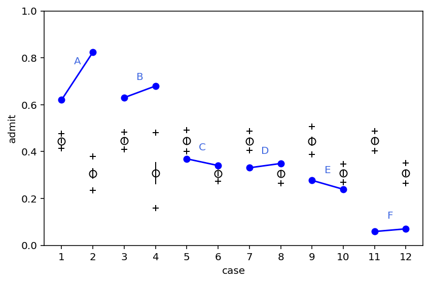
What above plot shows is that only for departments C & E, there was a lower rate of admissions for females. Now this is not in sync with what we observed earlier where the model was telling that females should expect an overall 14% lower chance of admission.

What is going on ?

Problem here is that male and females do not apply to same departments & departments also vary in their rate of admissions. Females do not apply to A & B that has higher rate of acceptance. Instead they applied to departments that have lower rate (10% of applicants) of acceptance.

Code 11.32

Changing the question to be asked -

Instead of asking -

What are the average probabilities of admission for females and males across all departments?

we are now going to ask -

What is the average difference in probability of admis- sion between females and males within departments?

# construct 6 unique indexes such that there are 2 entries per index
dept_id = np.repeat(np.arange(6), 2)


def model_11_8(gid, dept_id, N):
    def _generator():
        alpha = yield Root(tfd.Sample(tfd.Normal(loc=0.0, scale=1.5), sample_shape=2))
        delta = yield Root(tfd.Sample(tfd.Normal(loc=0.0, scale=1.5), sample_shape=6))

        p = tf.sigmoid(
            tf.squeeze(tf.gather(alpha, gid, axis=-1))
            + tf.squeeze(tf.gather(delta, dept_id, axis=-1))
        )

        A = yield tfd.Independent(
            tfd.Binomial(total_count=N, probs=p), reinterpreted_batch_ndims=1
        )

    return tfd.JointDistributionCoroutine(_generator, validate_args=True)


jdc_11_8 = model_11_8(tdf.gid, dept_id, tdf.applications)

init_state = [
    tf.zeros([NUMBER_OF_CHAINS, 2]),
    tf.zeros([NUMBER_OF_CHAINS, 6]),
]

bijectors = [tfb.Identity(), tfb.Identity()]

posterior_11_8, trace_11_8 = sample_posterior(
    jdc_11_8,
    observed_data=(tdf.admit,),
    params=["alpha", "delta"],
    init_state=init_state,
    bijectors=bijectors,
    num_samples=2000,
)

az.summary(trace_11_8, hdi_prob=0.89)

WARNING:tensorflow:5 out of the last 5 calls to <function run_hmc_chain at 0x7feb5545e7a0> triggered tf.function retracing. Tracing is expensive and the excessive number of tracings could be due to (1) creating @tf.function repeatedly in a loop, (2) passing tensors with different shapes, (3) passing Python objects instead of tensors. For (1), please define your @tf.function outside of the loop. For (2), @tf.function has experimental_relax_shapes=True option that relaxes argument shapes that can avoid unnecessary retracing. For (3), please refer to https://www.tensorflow.org/guide/function#controlling_retracing and https://www.tensorflow.org/api_docs/python/tf/function for  more details.

	mean	sd	hdi_5.5%	hdi_94.5%	mcse_mean	mcse_sd	ess_bulk	ess_tail	r_hat
alpha[0]	-0.721	0.580	-1.688	0.271	0.110	0.080	29.0	60.0	1.06
alpha[1]	-0.625	0.583	-1.600	0.391	0.111	0.080	29.0	58.0	1.06
delta[0]	1.304	0.583	0.427	2.398	0.110	0.080	29.0	59.0	1.06
delta[1]	1.257	0.586	0.348	2.313	0.110	0.080	30.0	66.0	1.06
delta[2]	0.042	0.582	-0.824	1.123	0.110	0.078	29.0	59.0	1.06
delta[3]	0.010	0.582	-0.840	1.118	0.110	0.079	29.0	65.0	1.06
delta[4]	-0.434	0.583	-1.302	0.670	0.110	0.078	29.0	62.0	1.06
delta[5]	-1.988	0.595	-2.931	-0.946	0.109	0.078	31.0	67.0	1.06

Code 11.33

Computing the contrast

diff_a = trace_11_8.posterior["alpha"][:, :, 0] - trace_11_8.posterior["alpha"][:, :, 1]
diff_p = tf.sigmoid(trace_11_8.posterior["alpha"][:, :, 0].values) - tf.sigmoid(
    trace_11_8.posterior["alpha"][:, :, 1].values
)

trace_11_8.posterior["diff_a"] = diff_a

coords = [trace_11_8.posterior.coords["chain"], trace_11_8.posterior.coords["draw"]]
trace_11_8.posterior["diff_p"] = xr.DataArray(
    diff_p, coords=coords, dims=["chain", "draw"]
)

az.summary(trace_11_8, hdi_prob=0.89)

	mean	sd	hdi_5.5%	hdi_94.5%	mcse_mean	mcse_sd	ess_bulk	ess_tail	r_hat
alpha[0]	-0.721	0.580	-1.688	0.271	0.110	0.080	29.0	60.0	1.06
alpha[1]	-0.625	0.583	-1.600	0.391	0.111	0.080	29.0	58.0	1.06
delta[0]	1.304	0.583	0.427	2.398	0.110	0.080	29.0	59.0	1.06
delta[1]	1.257	0.586	0.348	2.313	0.110	0.080	30.0	66.0	1.06
delta[2]	0.042	0.582	-0.824	1.123	0.110	0.078	29.0	59.0	1.06
delta[3]	0.010	0.582	-0.840	1.118	0.110	0.079	29.0	65.0	1.06
delta[4]	-0.434	0.583	-1.302	0.670	0.110	0.078	29.0	62.0	1.06
delta[5]	-1.988	0.595	-2.931	-0.946	0.109	0.078	31.0	67.0	1.06
diff_a	-0.097	0.085	-0.228	0.044	0.002	0.002	1174.0	969.0	1.00
diff_p	-0.021	0.019	-0.048	0.012	0.001	0.001	623.0	820.0	1.01

Code 11.34

pg = np.stack(
    list(
        map(
            lambda k: np.divide(
                d.applications[dept_id == k].values, d.applications[dept_id == k].sum()
            ),
            range(6),
        )
    ),
    axis=0,
).T
pg = pd.DataFrame(pg, index=["male", "female"], columns=d.dept.unique())
pg.round(2)

	A	B	C	D	E	F
male	0.88	0.96	0.35	0.53	0.33	0.52
female	0.12	0.04	0.65	0.47	0.67	0.48

Department A receives 88% of its applications from males. Department E receives 33% from males.

11.2 Poisson regression

Code 11.35

Binomial is good when the count is known but quite often it is not the case.

When the count goes extremely high then mean and variance of Binomial starts to become same and this is known as Poisson Distribution

y = tfd.Binomial(1000, probs=1 / 1000).sample((int(1e5),))
tf.reduce_mean(y).numpy(), np.var(y)

WARNING:tensorflow:6 out of the last 12 calls to <function _random_binomial at 0x7feb55cbd170> triggered tf.function retracing. Tracing is expensive and the excessive number of tracings could be due to (1) creating @tf.function repeatedly in a loop, (2) passing tensors with different shapes, (3) passing Python objects instead of tensors. For (1), please define your @tf.function outside of the loop. For (2), @tf.function has experimental_relax_shapes=True option that relaxes argument shapes that can avoid unnecessary retracing. For (3), please refer to https://www.tensorflow.org/guide/function#controlling_retracing and https://www.tensorflow.org/api_docs/python/tf/function for  more details.

(0.99741, 0.99274325)

Useful for binomial events for which the number of trials N is unknown or uncountably large.

Code 11.36

Counts of unique tool types for 10 historical Oceanic societies

d = RethinkingDataset.Kline.get_dataset()
d

	culture	population	contact	total_tools	mean_TU
0	Malekula	1100	low	13	3.2
1	Tikopia	1500	low	22	4.7
2	Santa Cruz	3600	low	24	4.0
3	Yap	4791	high	43	5.0
4	Lau Fiji	7400	high	33	5.0
5	Trobriand	8000	high	19	4.0
6	Chuuk	9200	high	40	3.8
7	Manus	13000	low	28	6.6
8	Tonga	17500	high	55	5.4
9	Hawaii	275000	low	71	6.6

To remember - Number of rows in count based models is not same as the sample size

Code 11.37

Here the outcome variable is total tools

We want to establish a relationship between log population and our outcome variable.

We also want to see the interaction between contact and log population

So first and foremost let’s create a column for log population

d["P"] = d.population.pipe(np.log).pipe(lambda x: (x - x.mean()) / x.std())
d["cid"] = (d.contact == "high").astype(int)

Code 11.38

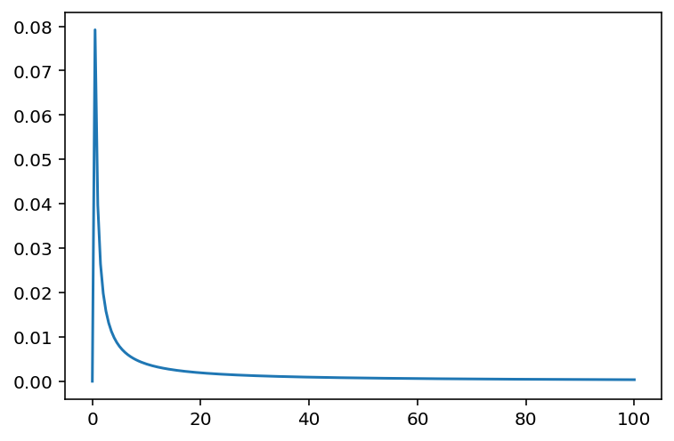
x = np.linspace(0, 100, 200)
plt.plot(x, tf.exp(tfd.LogNormal(loc=0.0, scale=10.0).log_prob(x)))
plt.show()

Code 11.39

a = tfd.Normal(loc=0.0, scale=10.0).sample(int(1e4))
lambda_ = tf.exp(a)
tf.reduce_mean(lambda_)

<tf.Tensor: shape=(), dtype=float32, numpy=2154870300000.0>

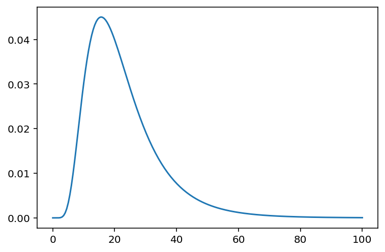
Code 11.40

x = np.linspace(0, 100, 200)
plt.plot(x, tf.exp(tfd.LogNormal(loc=3.0, scale=0.5).log_prob(x)))
plt.show()

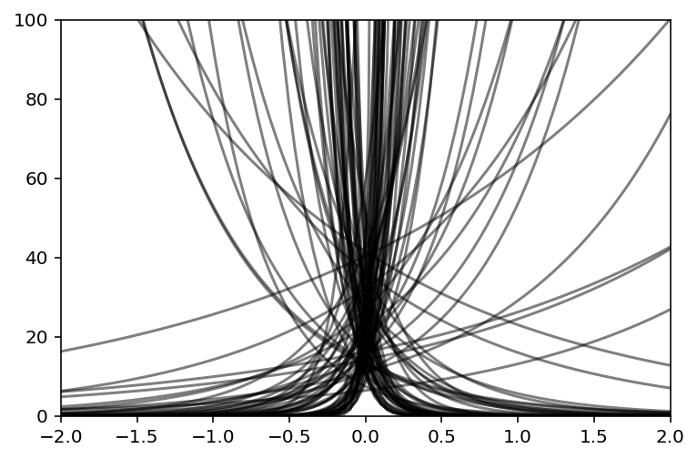
Code 11.41

N = 100
a = tfd.Normal(loc=3.0, scale=0.5).sample(N)
b = tfd.Normal(loc=0.0, scale=10.0).sample(N)
plt.subplot(xlim=(-2, 2), ylim=(0, 100))
x = np.linspace(-2, 2, 100)
for i in range(N):
    plt.plot(x, tf.exp(a[i] + b[i] * x), c="k", alpha=0.5)

Code 11.42

N = 100
a = tfd.Normal(loc=3.0, scale=0.5).sample(N).numpy()
b = tfd.Normal(loc=0.0, scale=0.2).sample(N).numpy()
plt.subplot(xlim=(-2, 2), ylim=(0, 100))
x = np.linspace(-2, 2, 100)
for i in range(N):
    plt.plot(x, tf.exp(a[i] + b[i] * x), c="k", alpha=0.5)

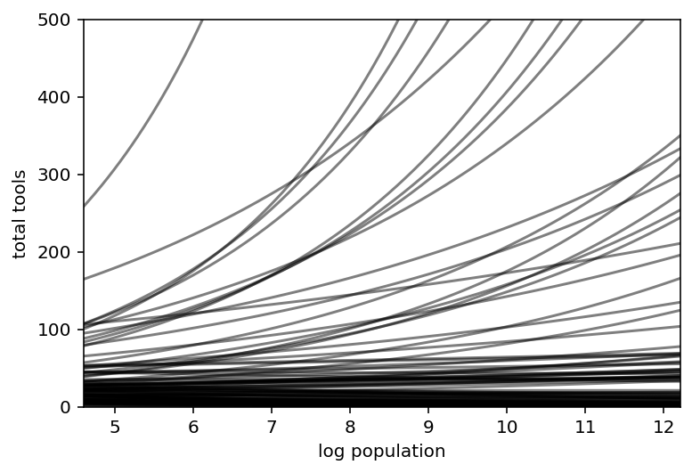
Code 11.43

x_seq = np.linspace(np.log(100), np.log(200000), num=100)
lambda_ = np.array(list(map(lambda x: np.exp(a + b * x), x_seq)))

plt.subplot(
    xlim=(np.min(x_seq).item(), np.max(x_seq).item()),
    ylim=(0, 500),
    xlabel="log population",
    ylabel="total tools",
)

plt.plot(x_seq, lambda_, c="k", alpha=0.5)
plt.show()

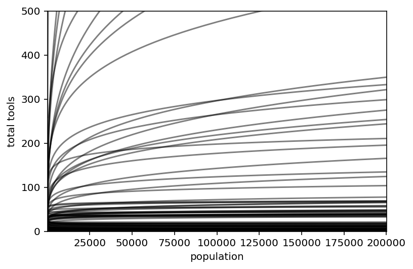
Code 11.44

plt.subplot(
    xlim=(np.min(np.exp(x_seq)).item(), np.max(np.exp(x_seq)).item()),
    ylim=(0, 500),
    xlabel="population",
    ylabel="total tools",
)
plt.plot(np.exp(x_seq), lambda_, c="k", alpha=0.5)
plt.show()

Code 11.45

# dat = dict(T=d.total_tools.values, P=d.P.values, cid=d.cid.values)

# d.total_tools.values

tdf = dataframe_to_tensors(
    "Kline", d, {"total_tools": tf.float32, "P": tf.float32, "cid": tf.int32}
)

# intercept only
def model_11_9():
    def _generator():
        alpha = yield Root(tfd.Sample(tfd.Normal(loc=3.0, scale=0.5), sample_shape=1))
        lambda_ = tf.exp(alpha[..., tf.newaxis])

        T = yield tfd.Independent(
            tfd.Poisson(rate=lambda_), reinterpreted_batch_ndims=1
        )

    return tfd.JointDistributionCoroutine(_generator, validate_args=False)


jdc_11_9 = model_11_9()

init_state = [3.0 * tf.zeros([NUMBER_OF_CHAINS])]

bijectors = [tfb.Identity()]

posterior_11_9, trace_11_9 = sample_posterior(
    jdc_11_9,
    observed_data=(tdf.total_tools,),
    init_state=init_state,
    bijectors=bijectors,
    params=["alpha"],
)

WARNING:tensorflow:From /opt/hostedtoolcache/Python/3.7.12/x64/lib/python3.7/site-packages/tensorflow_probability/python/distributions/distribution.py:342: calling Poisson.__init__ (from tensorflow_probability.python.distributions.poisson) with interpolate_nondiscrete is deprecated and will be removed after 2021-02-01.
Instructions for updating:
The `interpolate_nondiscrete` flag is deprecated; instead use `force_probs_to_zero_outside_support` (with the opposite sense).

WARNING:tensorflow:6 out of the last 6 calls to <function run_hmc_chain at 0x7feb5545e7a0> triggered tf.function retracing. Tracing is expensive and the excessive number of tracings could be due to (1) creating @tf.function repeatedly in a loop, (2) passing tensors with different shapes, (3) passing Python objects instead of tensors. For (1), please define your @tf.function outside of the loop. For (2), @tf.function has experimental_relax_shapes=True option that relaxes argument shapes that can avoid unnecessary retracing. For (3), please refer to https://www.tensorflow.org/guide/function#controlling_retracing and https://www.tensorflow.org/api_docs/python/tf/function for  more details.

# interaction model
def model_11_10(cid, P):
    def _generator():
        alpha = yield Root(tfd.Sample(tfd.Normal(loc=3.0, scale=0.5), sample_shape=2))
        beta = yield Root(tfd.Sample(tfd.Normal(loc=0.0, scale=0.2), sample_shape=2))

        lambda_ = tf.exp(
            tf.squeeze(tf.gather(alpha, cid, axis=-1))
            + tf.squeeze(tf.gather(beta, cid, axis=-1)) * P
        )

        T = yield tfd.Independent(
            tfd.Poisson(rate=lambda_), reinterpreted_batch_ndims=1
        )

    return tfd.JointDistributionCoroutine(_generator, validate_args=True)


jdc_11_10 = model_11_10(tdf.cid, tdf.P)

init_state = [tf.zeros([NUMBER_OF_CHAINS, 2]), tf.zeros([NUMBER_OF_CHAINS, 2])]

bijectors = [tfb.Identity(), tfb.Identity()]

posterior_11_10, trace_11_10 = sample_posterior(
    jdc_11_10,
    observed_data=(tdf.total_tools,),
    init_state=init_state,
    bijectors=bijectors,
    params=["alpha", "beta"],
)

Code 11.46

# We need to compute the log likelihood for model_11_9
# and then store it in the trace_11_9
#
# Reason to store it as it is expected by az.compare


def compute_and_store_log_likelihood_for_model_11_9():

    sample_alpha = posterior_11_9["alpha"]

    ds, _ = jdc_11_9.sample_distributions(value=[sample_alpha, None])

    log_likelihood_11_9 = ds[-1].distribution.log_prob(tdf.total_tools).numpy()

    # we need to insert this in the sampler_stats
    sample_stats_11_9 = trace_11_9.sample_stats

    coords = [
        sample_stats_11_9.coords["chain"],
        sample_stats_11_9.coords["draw"],
        np.arange(10),
    ]

    sample_stats_11_9["log_likelihood"] = xr.DataArray(
        log_likelihood_11_9,
        coords=coords,
        dims=["chain", "draw", "log_likelihood_dim_0"],
    )


compute_and_store_log_likelihood_for_model_11_9()

# We need to compute the log likelihood for model_11_10
# and then store it in the trace_11_10
#
# Reason to store it as it is expected by az.compare


def compute_and_store_log_likelihood_for_model_11_10():

    sample_alpha = posterior_11_10["alpha"]
    sample_beta = posterior_11_10["beta"]

    ds, _ = jdc_11_10.sample_distributions(value=[sample_alpha, sample_beta, None])

    log_likelihood_11_10 = ds[-1].distribution.log_prob(tdf.total_tools).numpy()

    # we need to insert this in the sampler_stats
    sample_stats_11_10 = trace_11_10.sample_stats

    coords = [
        sample_stats_11_10.coords["chain"],
        sample_stats_11_10.coords["draw"],
        np.arange(10),
    ]

    sample_stats_11_10["log_likelihood"] = xr.DataArray(
        log_likelihood_11_10,
        coords=coords,
        dims=["chain", "draw", "log_likelihood_dim_0"],
    )


compute_and_store_log_likelihood_for_model_11_10()

az.compare({"m11.9": trace_11_9, "m11.10": trace_11_10}, ic="loo")

/opt/hostedtoolcache/Python/3.7.12/x64/lib/python3.7/site-packages/arviz/stats/stats.py:695: UserWarning: Estimated shape parameter of Pareto distribution is greater than 0.7 for one or more samples. You should consider using a more robust model, this is because importance sampling is less likely to work well if the marginal posterior and LOO posterior are very different. This is more likely to happen with a non-robust model and highly influential observations.
  "Estimated shape parameter of Pareto distribution is greater than 0.7 for "
/opt/hostedtoolcache/Python/3.7.12/x64/lib/python3.7/site-packages/arviz/stats/stats.py:695: UserWarning: Estimated shape parameter of Pareto distribution is greater than 0.7 for one or more samples. You should consider using a more robust model, this is because importance sampling is less likely to work well if the marginal posterior and LOO posterior are very different. This is more likely to happen with a non-robust model and highly influential observations.
  "Estimated shape parameter of Pareto distribution is greater than 0.7 for "

	rank	loo	p_loo	d_loo	weight	se	dse	warning	loo_scale
m11.10	0	-42.49497	6.803545	0.0000	0.959477	6.249423	0.000000	True	log
m11.9	1	-70.61657	7.924030	28.1216	0.040523	16.114811	15.528969	True	log

Code 11.47

k = az.loo(trace_11_10, pointwise=True).pareto_k.values

cex = 1 + (k - np.min(k)) / (np.max(k) - np.min(k))
plt.scatter(
    d.P,
    d.total_tools,
    s=40 * cex,
    edgecolors=["none" if i == 1 else "b" for i in d.cid],
    facecolors=["none" if i == 0 else "b" for i in d.cid],
)
plt.gca().set(xlabel="log population (std)", ylabel="total tools", ylim=(0, 75))

# set up the horizontal axis values to compute predictions at
ns = 100
P_seq = np.linspace(-1.4, 3, num=ns)


# only using chain 0
sample_alpha = posterior_11_10["alpha"][0]
sample_beta = posterior_11_10["beta"][0]


def predict_and_plot(cid):
    term1 = tf.gather(sample_alpha, [cid], axis=-1)
    term2 = tf.gather(sample_beta, [cid], axis=-1) * P_seq
    lambda_ = tf.exp(term1 + term2)
    lmu = tf.reduce_mean(lambda_, 0)
    lci = tfp.stats.percentile(lambda_, (0.55, 94.5), 0)
    if cid == 0:
        plt.plot(P_seq, lmu, "k--", lw=1.5)
    else:
        plt.plot(P_seq, lmu, "k", lw=1.5)
    plt.fill_between(P_seq, lci[0], lci[1], color="k", alpha=0.2)


# make predictions when cid = 1 i.e. have low contact
predict_and_plot(0)
predict_and_plot(1)

/opt/hostedtoolcache/Python/3.7.12/x64/lib/python3.7/site-packages/arviz/stats/stats.py:695: UserWarning: Estimated shape parameter of Pareto distribution is greater than 0.7 for one or more samples. You should consider using a more robust model, this is because importance sampling is less likely to work well if the marginal posterior and LOO posterior are very different. This is more likely to happen with a non-robust model and highly influential observations.
  "Estimated shape parameter of Pareto distribution is greater than 0.7 for "

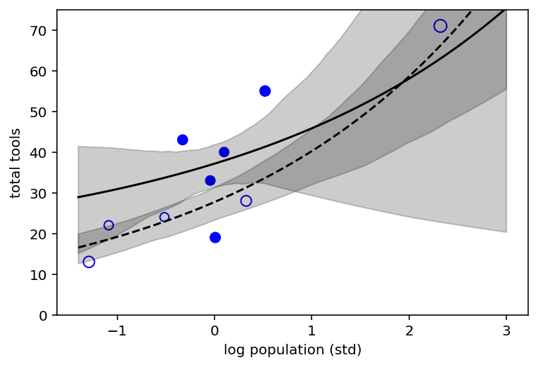
Open points are low contact societies and closed points are the high contact ones. Dashed curve is the posterior mean for low contact societies.

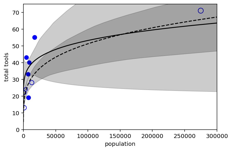
Code 11.48

cex = 1 + (k - np.min(k)) / (np.max(k) - np.min(k))

plt.scatter(
    d.population,
    d.total_tools,
    s=40 * cex,
    edgecolors=["none" if i == 1 else "b" for i in d.cid],
    facecolors=["none" if i == 0 else "b" for i in d.cid],
)
plt.gca().set(xlabel="population", ylabel="total tools", xlim=(0, 300000), ylim=(0, 75))

ns = 100
P_seq = np.linspace(-5, 3, num=ns)
# 1.53 is sd of log(population)
# 9 is mean of log(population)
pop_seq = np.exp(P_seq * 1.53 + 9)


def predict_and_plot(cid):
    term1 = tf.gather(sample_alpha, [cid], axis=-1)
    term2 = tf.gather(sample_beta, [cid], axis=-1) * P_seq
    lambda_ = tf.exp(term1 + term2)
    lmu = tf.reduce_mean(lambda_, 0)
    lci = tfp.stats.percentile(lambda_, (0.55, 94.5), 0)
    if cid == 0:
        plt.plot(pop_seq, lmu, "k--", lw=1.5)
    else:
        plt.plot(pop_seq, lmu, "k", lw=1.5)
    plt.fill_between(pop_seq, lci[0], lci[1], color="k", alpha=0.2)


# make predictions when cid = 1 i.e. have low contact
predict_and_plot(0)
predict_and_plot(1)

Code 11.49

tdf = dataframe_to_tensors(
    "Kline", d, {"total_tools": tf.float32, "population": tf.float32, "cid": tf.int32}
)


def model_11_11(cid, P):
    def _generator():
        g = yield Root(tfd.Sample(tfd.Exponential(1.0), sample_shape=1))
        beta = yield Root(tfd.Sample(tfd.Exponential(1.0), sample_shape=2))
        alpha = yield Root(tfd.Sample(tfd.Normal(loc=1.0, scale=1.0), sample_shape=2))

        term1 = tf.exp(tf.squeeze(tf.gather(alpha, cid, axis=-1)))
        term2 = tf.pow(P, tf.squeeze(tf.gather(beta, cid, axis=-1))) / g

        lambda_ = term1 + term2

        T = yield tfd.Independent(
            tfd.Poisson(rate=lambda_), reinterpreted_batch_ndims=1
        )

    return tfd.JointDistributionCoroutine(_generator, validate_args=True)


jdc_11_11 = model_11_11(tdf.cid, tdf.population)

11.2.2 Negative binomial (gamm-poisson) models

11.2.3 Example: Exposure and the offset

Code 11.50

num_days = 30
y = tfd.Poisson(rate=1.5).sample((num_days,))

Code 11.51

num_weeks = 4
y_new = tfd.Poisson(rate=0.5 * 7).sample((num_weeks,))

Code 11.52

y_all = np.concatenate([y, y_new])
exposure = np.concatenate([np.repeat(1, 30), np.repeat(7, 4)])
monastery = np.concatenate([np.repeat(0, 30), np.repeat(1, 4)])
d = pd.DataFrame.from_dict(dict(y=y_all, days=exposure, monastery=monastery))

d

	y	days	monastery
0	2.0	1	0
1	2.0	1	0
2	0.0	1	0
3	2.0	1	0
4	1.0	1	0
5	1.0	1	0
6	3.0	1	0
7	2.0	1	0
8	2.0	1	0
9	2.0	1	0
10	3.0	1	0
11	1.0	1	0
12	0.0	1	0
13	1.0	1	0
14	1.0	1	0
15	0.0	1	0
16	2.0	1	0
17	1.0	1	0
18	2.0	1	0
19	2.0	1	0
20	2.0	1	0
21	2.0	1	0
22	0.0	1	0
23	1.0	1	0
24	3.0	1	0
25	2.0	1	0
26	1.0	1	0
27	2.0	1	0
28	0.0	1	0
29	1.0	1	0
30	2.0	7	1
31	5.0	7	1
32	3.0	7	1
33	5.0	7	1

Code 11.53

# compute the offset
d["log_days"] = d.days.pipe(np.log)

tdf = dataframe_to_tensors(
    "Monastry", d, {"log_days": tf.float32, "monastery": tf.float32, "y": tf.float32}
)


def model_11_12(log_days, monastery):
    def _generator():
        a = yield Root(tfd.Sample(tfd.Normal(loc=0.0, scale=1.0), sample_shape=1))
        b = yield Root(tfd.Sample(tfd.Normal(loc=0.0, scale=1.0), sample_shape=1))

        lambda_ = tf.exp(log_days + a[..., tf.newaxis] + b[..., tf.newaxis] * monastery)

        T = yield tfd.Independent(
            tfd.Poisson(rate=lambda_), reinterpreted_batch_ndims=1
        )

    return tfd.JointDistributionCoroutine(_generator, validate_args=False)


jdc_11_12 = model_11_12(tdf.log_days, tdf.monastery)

init_state = [tf.zeros([NUMBER_OF_CHAINS]), tf.zeros([NUMBER_OF_CHAINS])]

bijectors = [tfb.Identity(), tfb.Identity()]


posterior_11_12, trace_11_12 = sample_posterior(
    jdc_11_12,
    observed_data=(tdf.y,),
    init_state=init_state,
    bijectors=bijectors,
    params=["alpha", "beta"],
)

Code 11.54

# using only the first chain
sample_alpha = posterior_11_12["alpha"][
    0:,
]
sample_beta = posterior_11_12["beta"][
    0:,
]

lambda_old = tf.exp(sample_alpha)
lambda_new = tf.exp(sample_alpha + sample_beta)

az.summary(
    az.from_dict({"lambda_old": lambda_old, "lambda_new": lambda_new}), hdi_prob=0.89
)

	mean	sd	hdi_5.5%	hdi_94.5%	mcse_mean	mcse_sd	ess_bulk	ess_tail	r_hat
lambda_old	1.417	0.206	1.085	1.754	0.016	0.012	160.0	214.0	1.0
lambda_new	0.567	0.122	0.376	0.735	0.007	0.005	265.0	381.0	1.0

11.3 Multinomial and categorical models

11.3.1 Predictors matched to outcomes

Code 11.55

Here we simulate career choice from three different careers, each with its own income trait. These traits are used to assign a score to each type of event. Then when the model is fit to the data, one of these scores is held constant, and the other two scores are estimated, using the known income traits

# simulate career choices among 500 individuals
N = 500  # number of individuals
income = np.array([1, 2, 5])  # expected income of each career
score = 0.5 * income  # scores for each career, based on income

# next line converts scores to probabilities
p = tf.nn.softmax(score)

# now simulate choice
# outcome career holds event type values, not counts
career = np.repeat(np.nan, N)  # empty vector of choices for each individual

# sample chosen career for each individual
for i in range(N):
    career[i] = tfd.Categorical(probs=p).sample()

career = career.astype(int)

Code 11.56

Categorical likelihood is a multinomial logistic regression distribution.

Each possible career will gets its own linear model with its own features.

def model_11_13(N, K, career_income):
    def _generator():
        print("==== start")
        # intercepts
        alpha = yield Root(
            tfd.Sample(tfd.Normal(loc=0.0, scale=1.0), sample_shape=(K - 1))
        )
        # association of income with choice
        beta = yield Root(tfd.Sample(tfd.HalfNormal(scale=0.5), sample_shape=1))

        print("alpja", alpha.shape)
        print("beta", beta.shape)

        s_1 = tf.gather(alpha, [0], axis=-1) + beta * career_income[0]
        s_2 = tf.gather(alpha, [1], axis=-1) + beta * career_income[1]
        s_3 = tf.zeros_like(s_1)  # pivot

        print("s1", s_1.shape)
        print("s2", s_2.shape)

        ts = tf.stack([s_1, s_2, s_3], axis=1)

        p = tf.nn.softmax(ts)

        print("p", p.shape)

        p_p = p
        print("==== end")

        career = yield tfd.Independent(
            tfd.Categorical(probs=p_p), reinterpreted_batch_ndims=1
        )

    return tfd.JointDistributionCoroutine(_generator, validate_args=True)

Code 11.57 (TODO - not able to make it work with 2 chains)

jdc_11_13 = model_11_13(N, 3, income)

jdc_11_13.sample(2)

==== start
alpja (2,)
beta (1,)
s1 (1,)
s2 (1,)
p (1, 3)
==== end
==== start
alpja (2, 2)
beta (2, 1)
s1 (2, 1)
s2 (2, 1)
p (2, 3, 1)
==== end

StructTuple(
  var0=<tf.Tensor: shape=(2, 2), dtype=float32, numpy=
    array([[ 0.9685273 , -0.84437585],
           [ 0.5235515 ,  0.16414931]], dtype=float32)>,
  var1=<tf.Tensor: shape=(2, 1), dtype=float32, numpy=
    array([[0.4134818 ],
           [0.18612705]], dtype=float32)>,
  var2=<tf.Tensor: shape=(2, 3), dtype=int32, numpy=
    array([[0, 0, 0],
           [0, 0, 0]], dtype=int32)>
)

NUMBER_OF_CHAINS_11_13 = 1

init_state = [tf.zeros([NUMBER_OF_CHAINS_11_13, 2]), tf.zeros([NUMBER_OF_CHAINS_11_13])]

bijectors = [tfb.Identity(), tfb.Identity()]

# Not working !

# posterior_11_13, trace_11_13 = sample_posterior(jdc_11_13,
#                                     observed_data=(career,),
#                                     init_state=init_state,
#                                     bijectors=bijectors,
#                                     params=["alpha", "beta"])

# az.summary(trace_11_13)

11.3.3 Multinomial in disguise as Poisson

Code 11.60

Multinomial in disguise as Poisson. The author shows a technique here on how to fit a multinomial/categorical model as a series of Poisson Likelihoods.

It is computationally easier to use Poisson rather than multinomial likelihoods

d = RethinkingDataset.UCBadmit.get_dataset()

d

	dept	applicant.gender	admit	reject	applications
1	A	male	512	313	825
2	A	female	89	19	108
3	B	male	353	207	560
4	B	female	17	8	25
5	C	male	120	205	325
6	C	female	202	391	593
7	D	male	138	279	417
8	D	female	131	244	375
9	E	male	53	138	191
10	E	female	94	299	393
11	F	male	22	351	373
12	F	female	24	317	341

tdf = dataframe_to_tensors(
    "UCBAdmit",
    d,
    {"applications": tf.float32, "admit": tf.float32, "reject": tf.float32},
)

Code 11.61

Using Poisson regression to model rate of admission & rate of rejection

def model_binomial(applications):
    def _generator():
        a = yield Root(tfd.Sample(tfd.Normal(loc=0.0, scale=1.5), sample_shape=1))
        logit = a[..., tf.newaxis]

        T = yield tfd.Independent(
            tfd.Binomial(total_count=applications, logits=logit),
            reinterpreted_batch_ndims=1,
        )

    return tfd.JointDistributionCoroutine(_generator, validate_args=False)


jdc_model_binom = model_binomial(tdf.applications)

init_state = [tf.zeros([NUMBER_OF_CHAINS])]

bijectors = [tfb.Identity()]

observed_data = (tdf.admit,)

posterior_model_binom, trace_model_binom = sample_posterior(
    jdc_model_binom,
    observed_data=observed_data,
    init_state=init_state,
    bijectors=bijectors,
    params=["alpha"],
)

# d["rej"] = d.reject


def model_pois(applications):
    def _generator():
        a = yield Root(tfd.Sample(tfd.Normal(loc=0.0, scale=1.5), sample_shape=2))
        lambda1 = tf.exp(tf.gather(a, 0, axis=-1))
        lambda2 = tf.exp(tf.gather(a, 1, axis=-1))

        A = yield tfd.Independent(
            tfd.Poisson(rate=lambda1[..., tf.newaxis]), reinterpreted_batch_ndims=1
        )

        R = yield tfd.Independent(
            tfd.Poisson(rate=lambda2[..., tf.newaxis]), reinterpreted_batch_ndims=1
        )

    return tfd.JointDistributionCoroutine(_generator, validate_args=True)


jdc_model_pois = model_pois(tdf.applications)

jdc_model_pois.sample(3)

init_state = [tf.zeros([NUMBER_OF_CHAINS, 2])]

bijectors = [tfb.Identity()]


observed_data = (tdf.admit, tdf.reject)

posterior_model_pois, trace_model_pois = sample_posterior(
    jdc_model_pois,
    observed_data=observed_data,
    init_state=init_state,
    bijectors=bijectors,
    params=["alpha"],
)

WARNING:tensorflow:5 out of the last 7 calls to <function random_poisson at 0x7feb55966e60> triggered tf.function retracing. Tracing is expensive and the excessive number of tracings could be due to (1) creating @tf.function repeatedly in a loop, (2) passing tensors with different shapes, (3) passing Python objects instead of tensors. For (1), please define your @tf.function outside of the loop. For (2), @tf.function has experimental_relax_shapes=True option that relaxes argument shapes that can avoid unnecessary retracing. For (3), please refer to https://www.tensorflow.org/guide/function#controlling_retracing and https://www.tensorflow.org/api_docs/python/tf/function for  more details.

Code 11.62

Inferred binomial probability of admission across the entire dataset

tf.math.sigmoid(np.median(posterior_model_pois["alpha"]))

<tf.Tensor: shape=(), dtype=float32, numpy=0.9947492>

Code 11.63

Inplied Poisson probability

k = tf.reduce_mean(posterior_model_pois["alpha"][0], 0)

a1 = k[0]
a2 = k[1]

tf.exp(a1) / (tf.exp(a1) + tf.exp(a2))

<tf.Tensor: shape=(), dtype=float32, numpy=0.39187136>

This is same as that of binomial model

11.4 Censoring and survival

Code 11.64

x2 = np.min(tfd.Uniform(low=1, high=100).sample((int(1e5), 2)), -1)
x5 = np.min(tfd.Uniform(low=1, high=100).sample((int(1e5), 5)), -1)

x2, x5

(array([76.54987 , 11.961508, 48.184395, ..., 23.755568, 14.266549,
         6.295066], dtype=float32),
 array([ 4.383093 , 38.237564 ,  2.7101636, ..., 45.11505  , 34.192856 ,
        35.747616 ], dtype=float32))

Code 11.65

N = 10
M = 2
x = np.sort(tfd.Uniform(low=1, high=100).sample((int(1e5), N)))[:, 1]

Code 11.66 - 11.69 (TODO)

d = RethinkingDataset.AustinCats.get_dataset()
d["adopt"] = (d.out_event == "Adoption").astype(int)
dat = dict(
    days_to_event=d.days_to_event.values,
    color_id=(d.color != "Black").astype(int).values,
    adopted=d.adopt.values,
)

previous

10. Big Entropy and The Generalized Linear Model

next

12. Monsters and Mixtures