9. Markov Chain Monte Carlo
Contents
![]()
9. Markov Chain Monte Carlo
# Install packages that are not installed in colab
try:
  import google.colab
  %pip install -q watermark
  %pip install git+https://github.com/ksachdeva/rethinking-tensorflow-probability.git
except:
  pass
%load_ext watermark
from functools import partial

from jax import ops
import jax.numpy as jnp

# Core
import numpy as np
import arviz as az
import pandas as pd
import tensorflow as tf
import tensorflow_probability as tfp

# visualization
import matplotlib.pyplot as plt

from rethinking.data import RethinkingDataset
from rethinking.data import dataframe_to_tensors
from rethinking.mcmc import sample_posterior


# aliases
tfd = tfp.distributions
Root = tfd.JointDistributionCoroutine.Root
2022-01-19 19:01:51.571884: W tensorflow/stream_executor/platform/default/dso_loader.cc:64] Could not load dynamic library 'libcudart.so.11.0'; dlerror: libcudart.so.11.0: cannot open shared object file: No such file or directory
%watermark -p numpy,tensorflow,tensorflow_probability,arviz,scipy,pandas,rethinking
numpy                 : 1.21.5
tensorflow            : 2.7.0
tensorflow_probability: 0.15.0
arviz                 : 0.11.4
scipy                 : 1.7.3
pandas                : 1.3.5
rethinking            : 0.1.0
# config of various plotting libraries
%config InlineBackend.figure_format = 'retina'
Introduction
9.1 Good King Markov and His island kingdom
Code 9.1
# Takes few minutes to run

num_weeks = int(1e5)
positions = np.repeat(0, num_weeks)
current = 10

coin_dist = tfd.Bernoulli(probs=0.5)
proposal_dist = tfd.Uniform(low=0.0, high=1.0)

for i in range(num_weeks):
    # record current position
    positions[i] = current

    # flip coin to generate proposal
    bern = coin_dist.sample().numpy()

    proposal = current + (bern * 2 - 1)

    # now make sure he loops around the archipelago
    proposal = np.where(proposal < 1, 10, proposal)
    proposal = np.where(proposal > 10, 1, proposal)

    # move?
    prob_move = proposal / current
    unif = proposal_dist.sample().numpy()
    current = np.where(unif < prob_move, proposal, current)
2022-01-19 19:01:53.728325: W tensorflow/stream_executor/platform/default/dso_loader.cc:64] Could not load dynamic library 'libcuda.so.1'; dlerror: libcuda.so.1: cannot open shared object file: No such file or directory
2022-01-19 19:01:53.728361: W tensorflow/stream_executor/cuda/cuda_driver.cc:269] failed call to cuInit: UNKNOWN ERROR (303)
---------------------------------------------------------------------------
KeyboardInterrupt                         Traceback (most recent call last)
/tmp/ipykernel_2260/2591419575.py in <module>
     23     # move?
     24     prob_move = proposal / current
---> 25     unif = proposal_dist.sample().numpy()
     26     current = np.where(unif < prob_move, proposal, current)

/opt/hostedtoolcache/Python/3.7.12/x64/lib/python3.7/site-packages/tensorflow_probability/python/distributions/distribution.py in sample(self, sample_shape, seed, name, **kwargs)
   1232     """
   1233     with self._name_and_control_scope(name):
-> 1234       return self._call_sample_n(sample_shape, seed, **kwargs)
   1235
   1236   def _call_sample_and_log_prob(self, sample_shape, seed, **kwargs):

/opt/hostedtoolcache/Python/3.7.12/x64/lib/python3.7/site-packages/tensorflow_probability/python/distributions/distribution.py in _call_sample_n(self, sample_shape, seed, **kwargs)
   1210         sample_shape, 'sample_shape')
   1211     samples = self._sample_n(
-> 1212         n, seed=seed() if callable(seed) else seed, **kwargs)
   1213     samples = tf.nest.map_structure(
   1214         lambda x: tf.reshape(x, ps.concat([sample_shape, ps.shape(x)[1:]], 0)),

/opt/hostedtoolcache/Python/3.7.12/x64/lib/python3.7/site-packages/tensorflow_probability/python/distributions/uniform.py in _sample_n(self, n, seed)
    154     shape = ps.concat([[n], self._batch_shape_tensor(
    155         low=low, high=high)], 0)
--> 156     samples = samplers.uniform(shape=shape, dtype=self.dtype, seed=seed)
    157     return low + self._range(low=low, high=high) * samples
    158

/opt/hostedtoolcache/Python/3.7.12/x64/lib/python3.7/site-packages/tensorflow_probability/python/internal/samplers.py in uniform(shape, minval, maxval, dtype, seed, name)
    282     seed = sanitize_seed(seed)
    283     return tf.random.stateless_uniform(
--> 284         shape=shape, seed=seed, minval=minval, maxval=maxval, dtype=dtype)

/opt/hostedtoolcache/Python/3.7.12/x64/lib/python3.7/site-packages/tensorflow/python/util/traceback_utils.py in error_handler(*args, **kwargs)
    148     filtered_tb = None
    149     try:
--> 150       return fn(*args, **kwargs)
    151     except Exception as e:
    152       filtered_tb = _process_traceback_frames(e.__traceback__)

/opt/hostedtoolcache/Python/3.7.12/x64/lib/python3.7/site-packages/tensorflow/python/util/dispatch.py in op_dispatch_handler(*args, **kwargs)
   1094       # Fallback dispatch system (dispatch v1):
   1095       try:
-> 1096         return dispatch_target(*args, **kwargs)
   1097       except (TypeError, ValueError):
   1098         # Note: convert_to_eager_tensor currently raises a ValueError, not a

/opt/hostedtoolcache/Python/3.7.12/x64/lib/python3.7/site-packages/tensorflow/python/ops/stateless_random_ops.py in stateless_random_uniform(shape, seed, minval, maxval, dtype, name, alg)
    342   with ops.name_scope(name, "stateless_random_uniform",
    343                       [shape, seed, minval, maxval]) as name:
--> 344     shape = tensor_util.shape_tensor(shape)
    345     if dtype.is_integer and minval is None:
    346       key, counter, alg = _get_key_counter_alg(seed, alg)

/opt/hostedtoolcache/Python/3.7.12/x64/lib/python3.7/site-packages/tensorflow/python/framework/tensor_util.py in shape_tensor(shape)
   1081       # not convertible to Tensors because of mixed content.
   1082       shape = tuple(map(tensor_shape.dimension_value, shape))
-> 1083   return ops.convert_to_tensor(shape, dtype=dtype, name="shape")
   1084
   1085

/opt/hostedtoolcache/Python/3.7.12/x64/lib/python3.7/site-packages/tensorflow/python/profiler/trace.py in wrapped(*args, **kwargs)
    161         with Trace(trace_name, **trace_kwargs):
    162           return func(*args, **kwargs)
--> 163       return func(*args, **kwargs)
    164
    165     return wrapped

/opt/hostedtoolcache/Python/3.7.12/x64/lib/python3.7/site-packages/tensorflow/python/framework/ops.py in convert_to_tensor(value, dtype, name, as_ref, preferred_dtype, dtype_hint, ctx, accepted_result_types)
   1584   if dtype is not None:
   1585     dtype = dtypes.as_dtype(dtype)
-> 1586   if isinstance(value, Tensor):
   1587     if dtype is not None and not dtype.is_compatible_with(value.dtype):
   1588       raise ValueError(

KeyboardInterrupt:
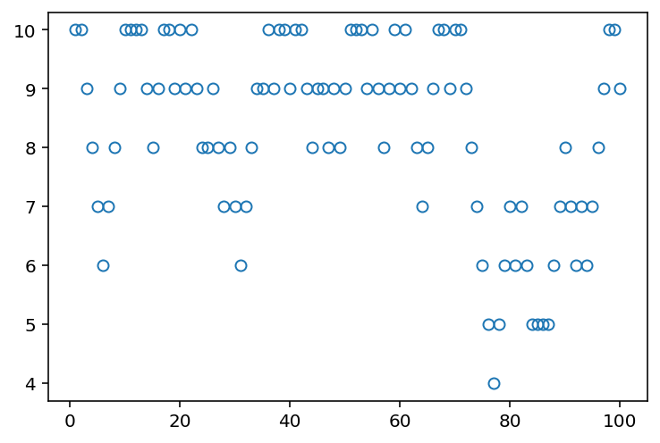
Code 9.2
plt.plot(range(1, 101), positions[:100], "o", mfc="none");
[<matplotlib.lines.Line2D at 0x14b8e3b10>]
Code 9.3
plt.hist(positions, bins=range(1, 12), rwidth=0.1, align="left");
(array([ 1877.,  3575.,  5267.,  7174.,  9175., 11077., 12910., 14408.,
        16217., 18320.]),
 array([ 1,  2,  3,  4,  5,  6,  7,  8,  9, 10, 11]),
 <BarContainer object of 10 artists>)
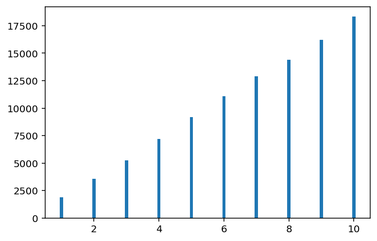
In above plot, horizontal axis is the islands (and their relative populations). Vertical axis is the number of weeks that King stayed at that island
9.2 Metropolis Algorithms
9.2.1 Gibbs sampling
9.2.2 High-dimensional problems
Code 9.4
What this section demonstrates is that as the number of dimensions increase the mass of the samples move away from the peak.
T = int(1e3)

_, ax = plt.subplots(2, 2, figsize=(8, 4))
plt.xlabel("Radial distance from the mode")


def build_and_plot(d, ax_p):
    loc = tf.cast(np.repeat(0, d), dtype=tf.float32)
    scale_diag = np.identity(d, dtype=np.float32)
    Y = tfd.MultivariateNormalDiag(loc=loc, scale_diag=scale_diag).sample((T,)).numpy()
    rad_dist = lambda Y: np.sqrt(np.sum(Y ** 2))
    Rd = list(map(lambda i: rad_dist(Y[i]), np.arange(T)))
    az.plot_kde(np.array(Rd), bw=0.18, label=f"Dim = {d}", ax=ax_p)


build_and_plot(1, ax[0][0])
build_and_plot(10, ax[0][1])
build_and_plot(100, ax[1][0])
build_and_plot(1000, ax[1][1])
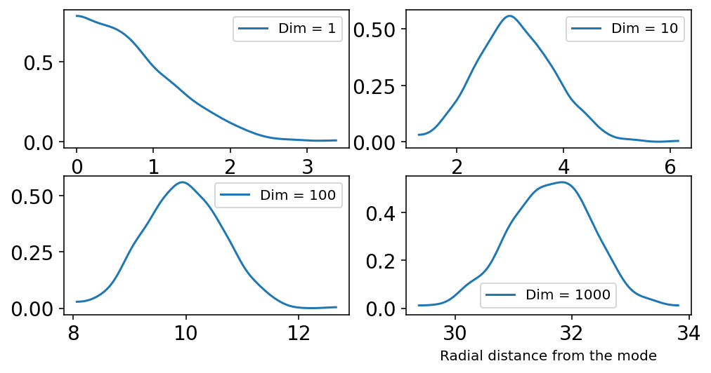
In the above plot, the horizontal axis shows Radial distance from the mode in the parameter space.
The peak in the above diagrams represent the amount of samples.
For Dim == 1, the peak is near 0
For Dim == 10, the peak is far from zero already
and so on …
The sampled points are in a thin, high-dimensional shell very far from the mode.
Because of above behavior (i.e. high dimensionsal space), the author suggests we need better MCMC algos than Metropolios and Gibbs
9.3 Hamiltonian Monte Carlo
Code 9.5
These next few cells will implement the Hamiltonian Monte Carlo algo. (Overthinking box in the chapter)
We need five things to do that -
A function named
Uthat returns the -ive log-prob of data at a current position (parameter value)A function named
grad_Uthat returns the gradient of the -ive log-prob at the current positionA step size
epsilonA count of leapfrog steps
LA starting position
current_q
Note - The position is a vector of parameter values & that the gradient also needs to return the vector of the same lenght.
## Note - change from the book here
#
# The book generates the test data in code 9.6 but I am going to generate it here


def generate_test_data():
    # test data
    _SEED = 7

    seed = tfp.util.SeedStream(seed=_SEED, salt="Testdata")
    y = tfd.Normal(loc=0.0, scale=1.0).sample(50, seed=seed()).numpy()
    x = tfd.Normal(loc=0.0, scale=1.0).sample(50, seed=seed()).numpy()

    # standardize the data
    y = (y - np.mean(y)) / np.std(y)
    x = (x - np.mean(x)) / np.std(x)

    return x, y


x, y = generate_test_data()

y
array([ 0.12833239, -0.22964787, -0.40774608, -0.30924067, -0.75710726,
       -1.12151   ,  0.54429084,  0.20373885,  0.5373924 ,  2.2354805 ,
       -0.55821157,  0.8479281 , -0.01069919, -2.2879438 ,  2.1183472 ,
        0.5721366 ,  1.5381907 , -2.4450817 , -0.15067661,  0.0314163 ,
       -0.06329995, -1.5469027 ,  0.6112922 , -0.6234371 ,  0.7724736 ,
        0.31413972,  2.2127857 , -0.30521753, -0.06263847,  0.60814875,
        1.7873812 , -0.23929906, -0.1567227 , -0.09433585, -0.25074163,
        0.3817731 , -1.289493  , -0.03346271, -0.25672948, -0.02745551,
        1.6410016 , -1.2717627 , -0.18327089,  0.6673328 , -0.7348228 ,
       -0.5346852 , -1.177903  , -0.9149043 , -0.3239217 ,  0.6152883 ],
      dtype=float32)
def U(q, a=0.0, b=1.0, k=0.0, d=1.0):
    muy = q[0]
    mux = q[1]

    logprob_y = tf.reduce_sum(tfd.Normal(loc=muy, scale=1.0).log_prob(y)).numpy()
    logprob_x = tf.reduce_sum(tfd.Normal(loc=mux, scale=1.0).log_prob(x)).numpy()

    logprob_muy = tfd.Normal(loc=a, scale=b).log_prob(muy).numpy()
    logprob_mux = tfd.Normal(loc=k, scale=d).log_prob(mux).numpy()

    return -(logprob_y + logprob_x + logprob_muy + logprob_mux)
Code 9.6
def U_gradient(q, a=0.0, b=1.0, k=0.0, d=1.0):
    muy = q[0]
    mux = q[1]
    G1 = np.sum(y - muy) + (a - muy) / b ** 2  # dU/dmuy
    G2 = np.sum(x - mux) + (k - mux) / b ** 2  # dU/dmux
    return np.stack([-G1, -G2])  # negative bc energy is neg-log-prob
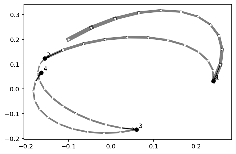
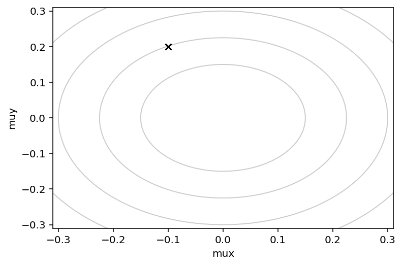
Code 9.7, 9.8, 9.9 & 9.10
Q = {}
Q["q"] = np.array([-0.1, 0.2])
pr = 0.31
plt.subplot(ylabel="muy", xlabel="mux", xlim=(-pr, pr), ylim=(-pr, pr))
step = 0.03
L = 11  # 0.03/28 for U-turns --- 11 for working example
n_samples = 4
path_col = (0, 0, 0, 0.5)
for r in 0.075 * np.arange(2, 6):
    plt.gca().add_artist(plt.Circle((0, 0), r, alpha=0.2, fill=False))
plt.scatter(Q["q"][0], Q["q"][1], c="k", marker="x", zorder=4)
<matplotlib.collections.PathCollection at 0x14bd51d50>
def HMC2(U, grad_U, epsilon, L, current_q):
    q = current_q

    # Random flick - p is the momentum
    p = tfd.Normal(loc=0.0, scale=1.0).sample(q.shape[0]).numpy()
    current_p = p

    # Make a half step for momentum at the begining
    p = p - epsilon * grad_U(q) / 2

    # initialize bookkeeping - saves trajectory
    qtraj = jnp.full((L + 1, q.shape[0]), np.nan)
    ptraj = qtraj

    qtraj = ops.index_update(qtraj, 0, current_q)
    ptraj = ops.index_update(ptraj, 0, p)

    # Alternate full steps for position and momentum
    for i in range(L):
        q = q + epsilon * p  # Full step for the position
        # Make a full step for the momentum, except at end of trajectory
        if i != (L - 1):
            p = p - epsilon * grad_U(q)
            ptraj = ops.index_update(ptraj, i + 1, p)
        qtraj = ops.index_update(qtraj, i + 1, q)

    # Make a half step for momentum at the end
    p = p - epsilon * grad_U(q) / 2

    # ptraj[L] = p
    ptraj = ops.index_update(ptraj, L, p)

    # Negate momentum at end of trajectory to make the proposal symmetric
    p = -p
    # Evaluate potential and kinetic energies at start and end of trajectory
    current_U = U(current_q)
    current_K = np.sum(current_p ** 2) / 2
    proposed_U = U(q)
    proposed_K = np.sum(p ** 2) / 2
    # Accept or reject the state at end of trajectory, returning either
    # the position at the end of the trajectory or the initial position
    accept = 0
    runif = tfd.Uniform(low=0.0, high=1.0).sample().numpy()
    if runif < np.exp(current_U - proposed_U + current_K - proposed_K):
        new_q = q  # accept
        accept = 1
    else:
        new_q = current_q  # reject

    return {
        "q": new_q,
        "traj": qtraj,
        "ptraj": ptraj,
        "accept": accept,
        "dH": proposed_U + proposed_K - (current_U + current_K),
    }


for i in range(n_samples):
    Q = HMC2(U, U_gradient, step, L, Q["q"])
    if n_samples < 10:
        for j in range(L):
            K0 = np.sum(Q["ptraj"][j] ** 2) / 2
            plt.plot(
                Q["traj"][j : j + 2, 0],
                Q["traj"][j : j + 2, 1],
                c=path_col,
                lw=1 + 2 * K0,
            )
        plt.scatter(Q["traj"][:, 0], Q["traj"][:, 1], c="white", s=5, zorder=3)
        # for fancy arrows
        dx = Q["traj"][L, 0] - Q["traj"][L - 1, 0]
        dy = Q["traj"][L, 1] - Q["traj"][L - 1, 1]
        d = np.sqrt(dx ** 2 + dy ** 2)
        plt.annotate(
            "",
            (Q["traj"][L - 1, 0], Q["traj"][L - 1, 1]),
            (Q["traj"][L, 0], Q["traj"][L, 1]),
            arrowprops={"arrowstyle": "<-"},
        )
        plt.annotate(
            str(i + 1),
            (Q["traj"][L, 0], Q["traj"][L, 1]),
            xytext=(3, 3),
            textcoords="offset points",
        )
    plt.scatter(
        Q["traj"][L + 1, 0],
        Q["traj"][L + 1, 1],
        c=("red" if np.abs(Q["dH"]) > 0.1 else "black"),
        zorder=4,
    )
WARNING:absl:No GPU/TPU found, falling back to CPU. (Set TF_CPP_MIN_LOG_LEVEL=0 and rerun for more info.)