5. The Many Variables & The Spurious Waffles¶

# Install packages that are not installed in colab
try:
  import google.colab
  %pip install --upgrade daft
  %pip install causalgraphicalmodels
  %pip install watermark
  %pip install git+https://github.com/ksachdeva/rethinking-tensorflow-probability.git
except:
  pass

%load_ext watermark

# Core
import numpy as np
import arviz as az
import pandas as pd
import tensorflow as tf
import tensorflow_probability as tfp

# visualization
import daft
import matplotlib.pyplot as plt
from causalgraphicalmodels import CausalGraphicalModel

from rethinking.data import RethinkingDataset
from rethinking.data import dataframe_to_tensors
from rethinking.mcmc import sample_posterior


# aliases
tfd = tfp.distributions
tfb = tfp.bijectors
Root = tfd.JointDistributionCoroutine.Root

2022-01-19 18:55:00.860760: W tensorflow/stream_executor/platform/default/dso_loader.cc:64] Could not load dynamic library 'libcudart.so.11.0'; dlerror: libcudart.so.11.0: cannot open shared object file: No such file or directory
2022-01-19 18:55:00.860796: I tensorflow/stream_executor/cuda/cudart_stub.cc:29] Ignore above cudart dlerror if you do not have a GPU set up on your machine.

%watermark -p numpy,tensorflow,tensorflow_probability,arviz,scipy,pandas,daft,causalgraphicalmodels,rethinking

numpy                 : 1.21.5
tensorflow            : 2.7.0
tensorflow_probability: 0.15.0
arviz                 : 0.11.4
scipy                 : 1.7.3
pandas                : 1.3.5
daft                  : 0.1.2
causalgraphicalmodels : 0.0.4
rethinking            : 0.1.0

# config of various plotting libraries
%config InlineBackend.figure_format = 'retina'

5.1 Spurious association¶

Code 5.1¶

The chapter is going to use 2 predictor variables - Marriage Rate & Median Age at Marriage to predict the divorce rate. Here we start with the first predictor variable - Median Age at Marriage

Loading the dataset and standardizing the variables of interest (i.e. median age at marriage and divorce rate)

d = RethinkingDataset.WaffleDivorce.get_dataset()

# standardize variables
d["A"] = d.MedianAgeMarriage.pipe(lambda x: (x - x.mean()) / x.std())
d["D"] = d.Divorce.pipe(lambda x: (x - x.mean()) / x.std())

Code 5.2¶

Here is the description of the linear regression model that use Median Age as the predictor variable.

\(D_i \sim Normal(\mu_i,\sigma)\)

\(\mu_i = \alpha + \beta_AA_i\)

\(\alpha \sim Normal(0,0.2)\)

\(\beta_A \sim Normal(0,0.5)\)

\(\sigma \sim Exponential(1)\)

We have standardized both D and A this means that the intercept (\(\alpha\)) should be close to zero.

A slope (\(\beta_A\)) of 1 would then imply that a change in one standard deviation in marriage rate is associated with change of one standard deviation in divorce.

Below we compute the standard deviation in median age

d.MedianAgeMarriage.std()

1.2436303013880823

This means that when \(\beta_A\) is 1 then we expect a change of 1.2 years in median age at marriage is associated with 1 full standard deviation of the divorce rate.

Code 5.3¶

Define the model and compute the posterior

tdf = dataframe_to_tensors("WaffleDivorce", d, ["A", "D"])


def model_5_1(median_age_data):
    def _generator():
        alpha = yield Root(
            tfd.Sample(tfd.Normal(loc=0.0, scale=0.2, name="alpha"), sample_shape=1)
        )
        betaA = yield Root(
            tfd.Sample(tfd.Normal(loc=0.0, scale=0.5, name="betaA"), sample_shape=1)
        )
        sigma = yield Root(
            tfd.Sample(tfd.Exponential(rate=1.0, name="sigma"), sample_shape=1)
        )

        mu = alpha + betaA * median_age_data

        divorce = yield tfd.Independent(
            tfd.Normal(loc=mu, scale=sigma, name="divorce"), reinterpreted_batch_ndims=1
        )

    return tfd.JointDistributionCoroutine(_generator, validate_args=True)


jdc_5_1 = model_5_1(tdf.A)

posterior_5_1, trace_5_1 = sample_posterior(
    jdc_5_1,
    observed_data=(tdf.D,),
    bijectors=[tfb.Identity(), tfb.Identity(), tfb.Exp()],
    params=["alpha", "betaA", "sigma"],
)

2022-01-19 18:55:03.766926: W tensorflow/stream_executor/platform/default/dso_loader.cc:64] Could not load dynamic library 'libcuda.so.1'; dlerror: libcuda.so.1: cannot open shared object file: No such file or directory
2022-01-19 18:55:03.766963: W tensorflow/stream_executor/cuda/cuda_driver.cc:269] failed call to cuInit: UNKNOWN ERROR (303)
2022-01-19 18:55:03.766987: I tensorflow/stream_executor/cuda/cuda_diagnostics.cc:156] kernel driver does not appear to be running on this host (fv-az272-145): /proc/driver/nvidia/version does not exist
2022-01-19 18:55:03.767320: I tensorflow/core/platform/cpu_feature_guard.cc:151] This TensorFlow binary is optimized with oneAPI Deep Neural Network Library (oneDNN) to use the following CPU instructions in performance-critical operations:  AVX2 FMA
To enable them in other operations, rebuild TensorFlow with the appropriate compiler flags.

Code 5.4¶

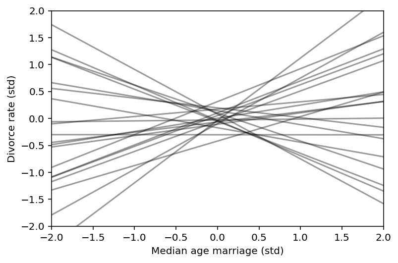
Before we do posterior analysis let’s check our priors

# Below we are using the value of A (median age)
A = tf.constant([-2, 2], dtype=tf.float32)
jdc_5_1_prior = model_5_1(A)
prior_pred_samples = jdc_5_1_prior.sample(1000)

prior_alpha = prior_pred_samples[0]
prior_beta = prior_pred_samples[1]
prior_sigma = prior_pred_samples[2]

ds, samples = jdc_5_1_prior.sample_distributions(
    value=[prior_alpha, prior_beta, prior_sigma, None]
)

mu = ds[-1].distribution.loc

plt.subplot(xlim=(-2, 2), ylim=(-2, 2))
for i in range(20):
    plt.plot([-2, 2], mu[i], "k", alpha=0.4)

plt.xlabel("Median age marriage (std)")
plt.ylabel("Divorce rate (std)");

../_images/05_the_many_variables_and_the_spurious_waffles_17_0.png

Code 5.5¶

Now for the posterior predictions.

sample_alpha = posterior_5_1["alpha"][0]
sample_betaA = posterior_5_1["betaA"][0]
sample_sigma = posterior_5_1["sigma"][0]

A_seq = tf.linspace(start=-3.0, stop=3.2, num=30)
A_seq = tf.cast(A_seq, dtype=tf.float32)

# we are creating a new model for the test values
jdc_5_1_test = model_5_1(A_seq)

# we will sample it using the trace_5_1
ds, samples = jdc_5_1_test.sample_distributions(
    value=[sample_alpha, sample_betaA, sample_sigma, None]
)

mu_pred = ds[-1].distribution.loc

mu_mean = tf.reduce_mean(mu_pred, 0)
mu_PI = tfp.stats.percentile(mu_pred, q=(5.5, 94.5), axis=0)

# plot it all
az.plot_pair(d[["A", "D"]].to_dict(orient="list"))
plt.fill_between(A_seq, mu_PI[0], mu_PI[1], color="k", alpha=0.2)
plt.plot(A_seq, mu_mean, "k");

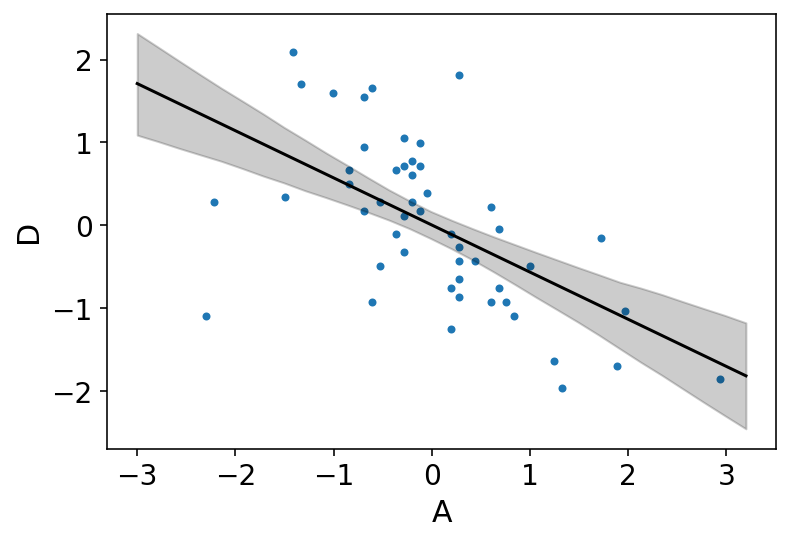
../_images/05_the_many_variables_and_the_spurious_waffles_20_0.png

Above plot is showing that the influence of age at marriage is strongly negative with divorce rate

Code 5.6¶

We can now model a simple regression for the Mariage rate as well.

d["M"] = d.Marriage.pipe(lambda x: (x - x.mean()) / x.std())

tdf = dataframe_to_tensors("WaffleDivorce", d, ["A", "D", "M"])


def model_5_2(marriage_rate_data):
    def _generator():
        alpha = yield Root(
            tfd.Sample(tfd.Normal(loc=0.0, scale=0.2, name="alpha"), sample_shape=1)
        )
        betaM = yield Root(
            tfd.Sample(tfd.Normal(loc=0.0, scale=0.5, name="betaM"), sample_shape=1)
        )
        sigma = yield Root(
            tfd.Sample(tfd.Exponential(rate=1.0, name="sigma"), sample_shape=1)
        )

        mu = alpha + betaM * marriage_rate_data

        divorce = yield tfd.Independent(
            tfd.Normal(loc=mu, scale=sigma, name="divorce"), reinterpreted_batch_ndims=1
        )

    return tfd.JointDistributionCoroutine(_generator, validate_args=True)


jdc_5_2 = model_5_2(tdf.M)

posterior_5_2, trace_5_2 = sample_posterior(
    jdc_5_2, observed_data=(tdf.D,), params=["alpha", "betaM", "sigma"]
)

sample_alpha = posterior_5_2["alpha"][0]
sample_betaM = posterior_5_2["betaM"][0]
sample_sigma = posterior_5_2["sigma"][0]

M_seq = tf.linspace(start=-3.0, stop=3.2, num=30)
M_seq = tf.cast(M_seq, tf.float32)

# we are creating a new model for the test values
jdc_5_2_test = model_5_2(M_seq)

# we will sample it using the trace_5_1
ds, samples = jdc_5_2_test.sample_distributions(
    value=[sample_alpha, sample_betaM, sample_sigma, None]
)

mu_pred = ds[-1].distribution.loc

mu_mean = tf.reduce_mean(mu_pred, 0)
mu_PI = tfp.stats.percentile(mu_pred, q=(5.5, 94.5), axis=0)

# plot it all
az.plot_pair(d[["M", "D"]].to_dict(orient="list"))
plt.fill_between(M_seq, mu_PI[0], mu_PI[1], color="k", alpha=0.2)
plt.plot(M_seq, mu_mean, "k");

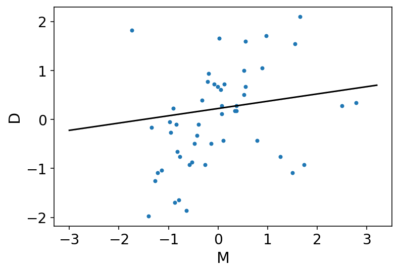
../_images/05_the_many_variables_and_the_spurious_waffles_24_0.png

Above plot is showing that the influence of marriage rate is strongly positive with divorce rate

Code 5.7¶

Author suggests that merely comparing parameter means between bivariate regressions is no way to decide which predictor is better. They may be independent, or related or could eliminate other.

How do we understand all this ?

He explains that here we may want to think causally.

Few interesting assumptions (or rather deductions) -

a) Age has a direct impact on Divorce rate as people may grow incompatible with the parter

b) Marriage Rate has a direct impact on Divorce rate for obvious reason (more marriages => more divorce)

c) Finally, Age has an impact on Marriage Rate because there are more young people

Another way to represent above is :

A -> D

M -> D

A -> M

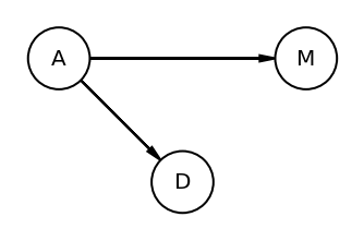
and yet another way is to use DAG (Directed Acyclic Graphs)

dag5_1 = CausalGraphicalModel(
    nodes=["A", "D", "M"], edges=[("A", "D"), ("A", "M"), ("M", "D")]
)
pgm = daft.PGM()
coordinates = {"A": (0, 0), "D": (1, 1), "M": (2, 0)}
for node in dag5_1.dag.nodes:
    pgm.add_node(node, node, *coordinates[node])
for edge in dag5_1.dag.edges:
    pgm.add_edge(*edge)
pgm.render()
plt.gca().invert_yaxis()

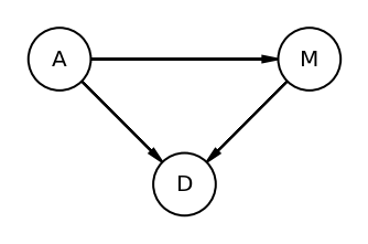
../_images/05_the_many_variables_and_the_spurious_waffles_27_0.png

Above DAG clearly shows that A impacts D directly and indirectly (i.e. via M)

The author used “total influence”. What is meant by total is that we need to account for every path from A to D.

MEDIATION - Let’s say that A did not directly influenced D; rather it did it via M. This type of relationship is called Mediation

Author raises many interesting questions here. He asks if there is indeed a direct effect of marriage rate or rather is age at marriage just driving both, creating a spurious coorelation between marriage rate and divorce rate

Code 5.8¶

Checking conditional indpendencies

# Note - There is no explicity code section for drawing the second DAG
# but the figure appears in the book and hence drawing it as well
dag5_2 = CausalGraphicalModel(nodes=["A", "D", "M"], edges=[("A", "D"), ("A", "M")])
pgm = daft.PGM()
coordinates = {"A": (0, 0), "D": (1, 1), "M": (2, 0)}
for node in dag5_2.dag.nodes:
    pgm.add_node(node, node, *coordinates[node])
for edge in dag5_2.dag.edges:
    pgm.add_edge(*edge)
pgm.render()
plt.gca().invert_yaxis()

../_images/05_the_many_variables_and_the_spurious_waffles_30_0.png

DMA_dag2 = CausalGraphicalModel(nodes=["A", "D", "M"], edges=[("A", "D"), ("A", "M")])
all_independencies = DMA_dag2.get_all_independence_relationships()
for s in all_independencies:
    if all(
        t[0] != s[0] or t[1] != s[1] or not t[2].issubset(s[2])
        for t in all_independencies
        if t != s
    ):
        print(s)

('D', 'M', {'A'})

Code 5.9¶

Checking conditional indpenedencies in the DAG1

DMA_dag1 = CausalGraphicalModel(
    nodes=["A", "D", "M"], edges=[("A", "D"), ("A", "M"), ("M", "D")]
)
all_independencies = DMA_dag1.get_all_independence_relationships()
for s in all_independencies:
    if all(
        t[0] != s[0] or t[1] != s[1] or not t[2].issubset(s[2])
        for t in all_independencies
        if t != s
    ):
        print(s)

Executing above cell should not display anything as in the DAG1 (where all nodes are connected to each other) there are no conditional indpedencies.

Code 5.10¶

def model_5_3(median_age_data, marriage_rate_data):
    def _generator():
        alpha = yield Root(
            tfd.Sample(tfd.Normal(loc=0.0, scale=0.2, name="alpha"), sample_shape=1)
        )
        betaA = yield Root(
            tfd.Sample(tfd.Normal(loc=0.0, scale=0.5, name="betaA"), sample_shape=1)
        )
        betaM = yield Root(
            tfd.Sample(tfd.Normal(loc=0.0, scale=0.5, name="betaM"), sample_shape=1)
        )
        sigma = yield Root(
            tfd.Sample(tfd.Exponential(rate=1.0, name="sigma"), sample_shape=1)
        )

        mu = alpha + betaA * median_age_data + betaM * marriage_rate_data

        divorce = yield tfd.Independent(
            tfd.Normal(loc=mu, scale=sigma, name="divorce"), reinterpreted_batch_ndims=1
        )

    return tfd.JointDistributionCoroutine(_generator, validate_args=True)


jdc_5_3 = model_5_3(tdf.A, tdf.M)

posterior_5_3, trace_5_3 = sample_posterior(
    jdc_5_3, observed_data=(tdf.D,), params=["alpha", "betaA", "betaM", "sigma"]
)

az.summary(trace_5_3, round_to=2, kind="stats", hdi_prob=0.89)

	mean	sd	hdi_5.5%	hdi_94.5%
alpha[0]	-0.01	0.11	-0.18	0.16
betaA[0]	-0.58	0.12	-0.78	-0.40
betaM[0]	-0.06	0.15	-0.30	0.18
sigma[0]	0.85	0.09	0.70	0.99

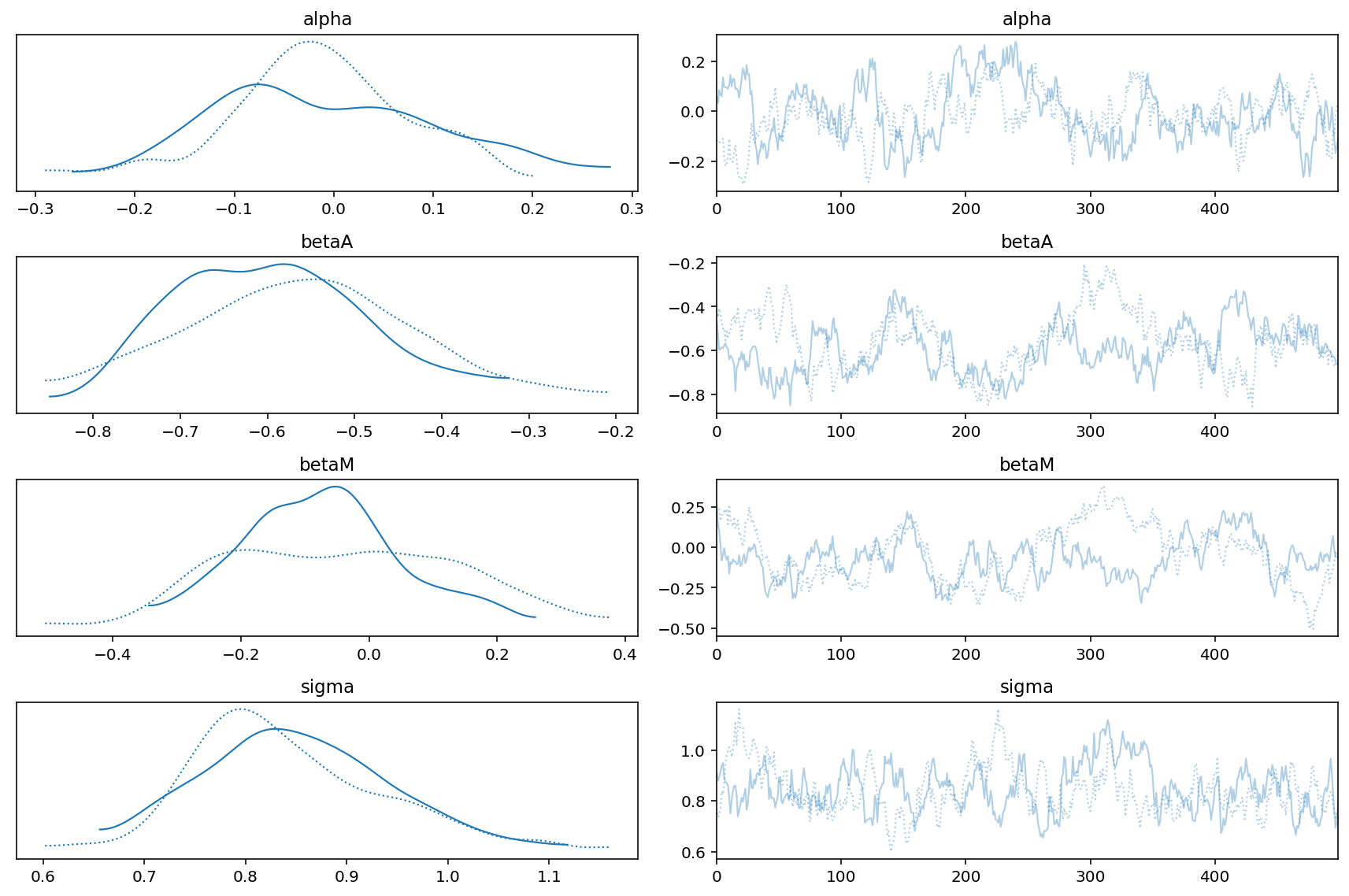
Let’s try to understand the above table generated by arviz.

In the model above, we had include both the predictors i.e. M & A. The weights of M i.e. betaM is approaching zero where as betaA is more or less unchanged.

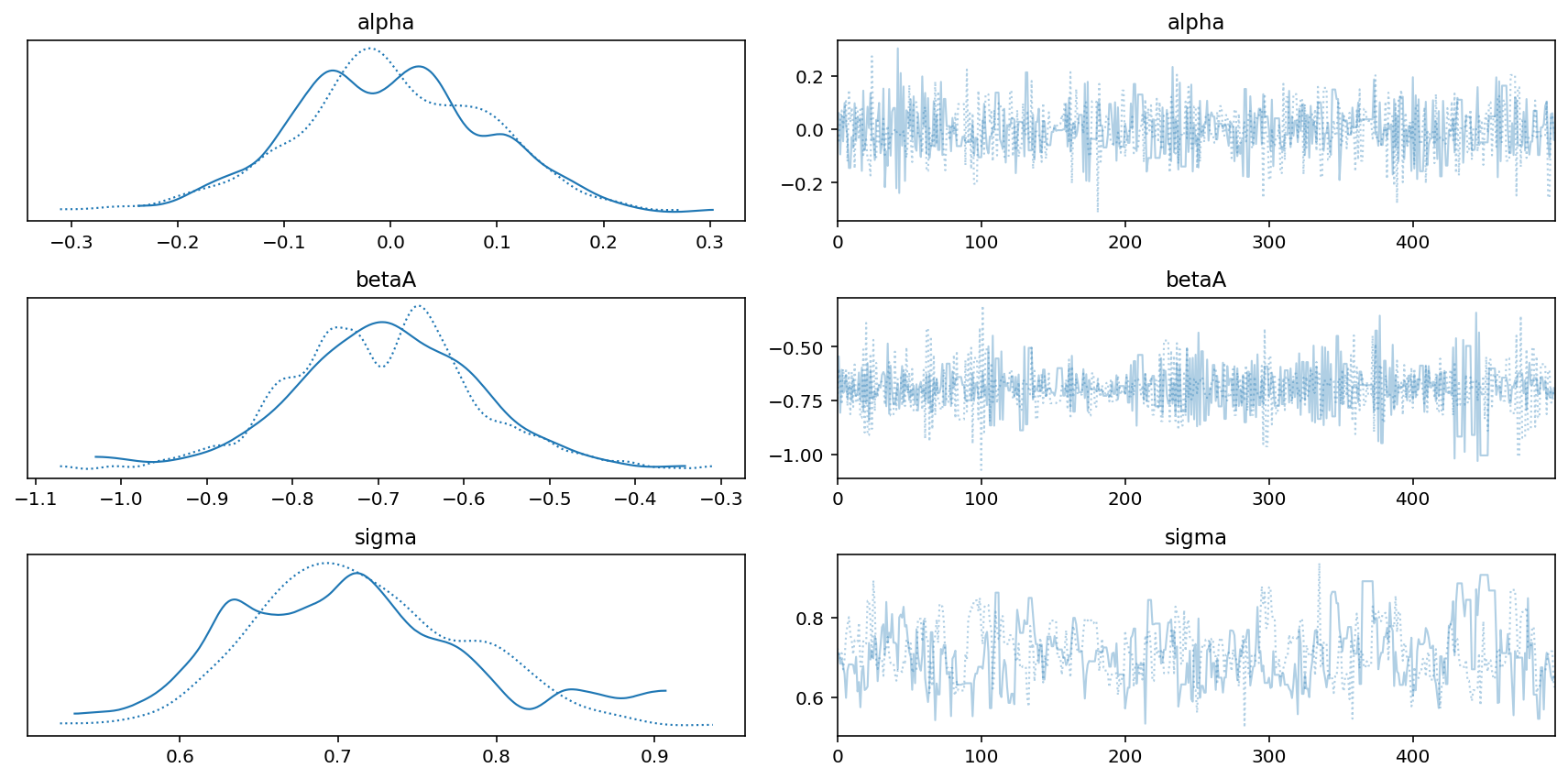
az.plot_trace(trace_5_3)
plt.tight_layout();

../_images/05_the_many_variables_and_the_spurious_waffles_39_0.png

Code 5.11¶

Here we will take the help of forest plot to compare the posteriors of various models that we have built so far

coeftab = {"m5.1": trace_5_1, "m5.2": trace_5_2, "m5.3": trace_5_3}

az.plot_forest(
    list(coeftab.values()),
    model_names=list(coeftab.keys()),
    combined=True,
    var_names=["betaA", "betaM"],
    hdi_prob=0.89,
);

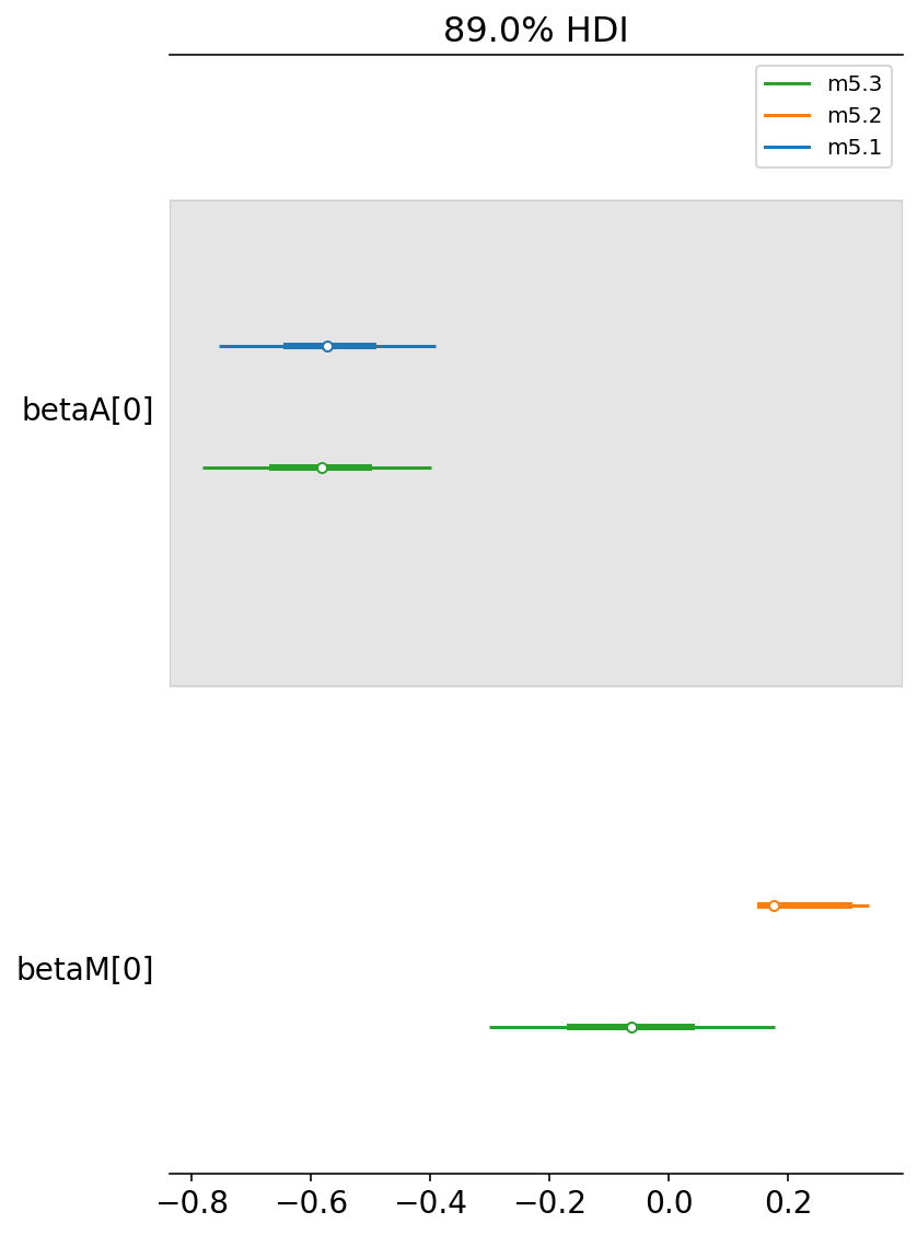
../_images/05_the_many_variables_and_the_spurious_waffles_41_0.png

Let’s learn how to read above plot

m5.1 is our first model where we had used betaA. If we compare it to m5.3 it is more or less at the same place.

whereas,

m5.2 is our second model where we had used betaM. If we compare it to m5.3, it is now closer to zero.

This is another way to read/plot what we saw in the arviz summary in Code 5.10

From all this, we can say that - once we know median age at marriage for a State, there is little or no additional predictive power in also knowing the rate of marriage in that state

Code 5.12 (TODO)¶

Possibly revisit this to do what professor has asked to do instead of just translating the code in the cell

N = 50  # number of simulated States
age = tfd.Normal(loc=0.0, scale=1.0).sample((N,))  # sim A
mar = tfd.Normal(loc=age, scale=1.0).sample()  # sim A -> M
div = tfd.Normal(loc=age, scale=1.0).sample()  # sim A -> D

Code 5.13¶

Following few cells are all about how to plot multivariate posteriors.

Previously we had only 1 predictor variable and hence a single scatterplot can convey a lot of information. Addition of regression lines and intervals also helped in estimating the size and uncertainity.

However, in the case multivariate regression we would have use other types of plots.

Author mentions that we need to also know how to select the proper type of plot for a given problem.

He explains 3 types of plots -

Predictor residual plots
Posterior prediction plots
Counterfactual plots

# we are first redefining our first model. It is exactly the same as m5_1


def model_5_4(median_age_data):
    def _generator():
        alpha = yield Root(
            tfd.Sample(tfd.Normal(loc=0.0, scale=0.2, name="alpha"), sample_shape=1)
        )
        betaA = yield Root(
            tfd.Sample(tfd.Normal(loc=0.0, scale=0.5, name="betaA"), sample_shape=1)
        )
        sigma = yield Root(
            tfd.Sample(tfd.Exponential(rate=1.0, name="sigma"), sample_shape=1)
        )

        mu = alpha + betaA * median_age_data

        M = yield tfd.Independent(
            tfd.Normal(loc=mu, scale=sigma, name="M"), reinterpreted_batch_ndims=1
        )

    return tfd.JointDistributionCoroutine(_generator, validate_args=True)


jdc_5_4 = model_5_4(tdf.A)

posterior_5_4, trace_5_4 = sample_posterior(
    jdc_5_4, observed_data=(tdf.D,), params=["alpha", "betaA", "sigma"]
)

az.plot_trace(trace_5_4)
plt.tight_layout();

../_images/05_the_many_variables_and_the_spurious_waffles_48_0.png

Code 5.14¶

First is Predictor residual plot

sample_alpha = posterior_5_4["alpha"][0]
sample_betaA = posterior_5_4["betaA"][0]
sample_sigma = posterior_5_4["sigma"][0]

ds, samples = jdc_5_4.sample_distributions(
    value=[sample_alpha, sample_betaA, sample_sigma, None]
)

mu_pred = ds[-1].distribution.loc

mu_mean = tf.reduce_mean(mu_pred, 0)
mu_resid = d.M.values - mu_mean

Code 5.15¶

Second is Posterior prediction plots

sample_alpha = posterior_5_3["alpha"][0]
sample_betaA = posterior_5_3["betaA"][0]
sample_betaM = posterior_5_3["betaM"][0]
sample_sigma = posterior_5_3["sigma"][0]

ds, samples = jdc_5_3.sample_distributions(
    value=[sample_alpha, sample_betaA, sample_betaM, sample_sigma, None]
)

mu_pred = ds[-1].distribution.loc

mu_mean = tf.reduce_mean(mu_pred, 0)
mu_PI = tfp.stats.percentile(mu_pred, q=(5.5, 94.5), axis=0).numpy()

# get the simulated D
D_sim = samples[-1]
D_PI = tfp.stats.percentile(D_sim, q=(5.5, 94.5), axis=0)

D_sim.shape

TensorShape([500, 50])

Code 5.16¶

Plot predictions against the observed

ax = plt.subplot(
    ylim=(float(mu_PI.min()), float(mu_PI.max())),
    xlabel="Observed divorce",
    ylabel="Predicted divorce",
)
plt.plot(d.D, mu_mean, "o")
x = np.linspace(mu_PI.min(), mu_PI.max(), 101)
plt.plot(x, x, "--")
for i in range(d.shape[0]):
    plt.plot([d.D[i]] * 2, mu_PI[:, i], "b")
fig = plt.gcf();

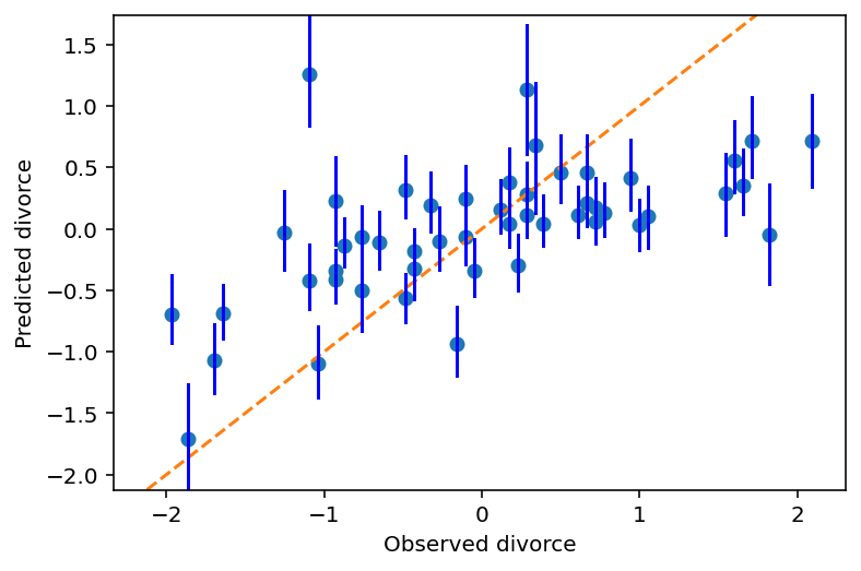
../_images/05_the_many_variables_and_the_spurious_waffles_54_0.png

The diagonal line shows perfect predictions.

Code 5.17¶

for i in range(d.shape[0]):
    if d.Loc[i] in ["ID", "UT", "RI", "ME"]:
        ax.annotate(
            d.Loc[i], (d.D[i], mu_mean[i]), xytext=(-25, -5), textcoords="offset pixels"
        )
fig

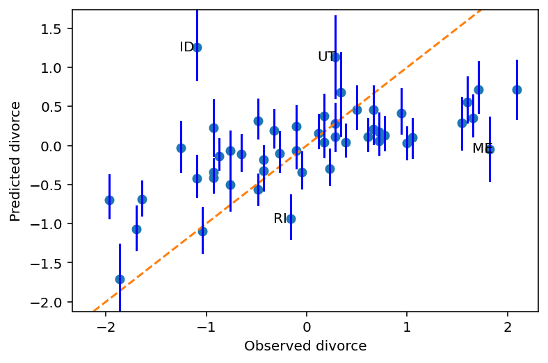
../_images/05_the_many_variables_and_the_spurious_waffles_57_0.png

Remember that the above graph is draw using m5_3 that had taken both predictor variables in account.

According to book, above figure shows - “Model under-predicts for States with very high divorce rate while it over-predicts for states with very low divorce rates.”

I am not able to interpret that :(

Some states, the ones which are labelled i.e. Idaho (ID), Utah (UT) have lower divorce rates because of religious regions.

Code 5.18¶

N = 100  # number of cases
# x_real as Gaussian with mean 0 and stddev 1
x_real = tfd.Normal(loc=0.0, scale=1.0).sample((N,))
# x_spur as Gaussian with mean=x_real
x_spur = tfd.Normal(loc=x_real, scale=1.0).sample()
# y as Gaussian with mean=x_real
y = tfd.Normal(loc=x_real, scale=1.0).sample()
# bind all together in data frame
d = pd.DataFrame({"y": y, "x_real": x_real, "x_spur": x_spur})

	y	x_real	x_spur
0	2.856022	1.029397	3.258285
1	0.325448	-0.343423	-1.713648
2	0.888222	0.720931	0.240602
3	-1.067678	-1.308793	-1.185875
4	-2.002595	-0.842671	-1.544350
...	...	...	...
95	2.892173	1.920939	2.521733
96	-0.738538	0.197148	0.888211
97	-2.505556	-2.660993	-3.071483
98	1.755759	0.732562	-0.445380
99	0.146894	1.098481	-1.387419

100 rows × 3 columns

Code 5.19¶

Third type of plot is called Counterfactual Plots

The simplest use of counterfactual plot is to see how the prediction changes as we change only one predictor at a time.

# Reloading the dataset

d = RethinkingDataset.WaffleDivorce.get_dataset()

# standardize variables
d["A"] = d.MedianAgeMarriage.pipe(lambda x: (x - x.mean()) / x.std())
d["D"] = d.Divorce.pipe(lambda x: (x - x.mean()) / x.std())
d["M"] = d.Marriage.pipe(lambda x: (x - x.mean()) / x.std())

tdf = dataframe_to_tensors("WaffleDivorce", d, ["A", "D", "M"])

def model_5_3_A(median_age_data, marriage_rate_data):
    def _generator():
        alpha = yield Root(
            tfd.Sample(tfd.Normal(loc=0.0, scale=0.2, name="alpha"), sample_shape=1)
        )
        betaA = yield Root(
            tfd.Sample(tfd.Normal(loc=0.0, scale=0.5, name="betaA"), sample_shape=1)
        )
        betaM = yield Root(
            tfd.Sample(tfd.Normal(loc=0.0, scale=0.5, name="betaM"), sample_shape=1)
        )
        sigma = yield Root(
            tfd.Sample(tfd.Exponential(rate=1.0, name="sigma"), sample_shape=1)
        )

        mu = alpha + betaA * median_age_data + betaM * marriage_rate_data

        divorce = yield tfd.Independent(
            tfd.Normal(loc=mu, scale=sigma, name="divorce"), reinterpreted_batch_ndims=1
        )

    return tfd.JointDistributionCoroutine(_generator, validate_args=True)


def model_5_X_M(median_age_data):
    def _generator():
        alphaM = yield Root(
            tfd.Sample(tfd.Normal(loc=0.0, scale=0.2, name="alphaM"), sample_shape=1)
        )
        betaAM = yield Root(
            tfd.Sample(tfd.Normal(loc=0.0, scale=0.5, name="betaAM"), sample_shape=1)
        )
        sigmaM = yield Root(
            tfd.Sample(tfd.Exponential(rate=1.0, name="sigmaM"), sample_shape=1)
        )

        mu_M = alphaM + betaAM * median_age_data

        M = yield tfd.Independent(
            tfd.Normal(loc=mu_M, scale=sigmaM, name="M"), reinterpreted_batch_ndims=1
        )

    return tfd.JointDistributionCoroutine(_generator, validate_args=True)


## First model
jdc_5_3_A = model_5_3_A(tdf.A, tdf.M)
posterior_5_3_A, trace_5_3_A = sample_posterior(
    jdc_5_3_A, observed_data=(tdf.D,), params=["alpha", "betaA", "betaM", "sigma"]
)

## Second model
jdc_5_X_M = model_5_X_M(tdf.A)
posterior_5_X_M, trace_5_X_M = sample_posterior(
    jdc_5_X_M, observed_data=(tdf.M,), params=["alpha", "betaA", "sigma"]
)

WARNING:tensorflow:5 out of the last 5 calls to <function run_hmc_chain at 0x7fe4ae8e4e60> triggered tf.function retracing. Tracing is expensive and the excessive number of tracings could be due to (1) creating @tf.function repeatedly in a loop, (2) passing tensors with different shapes, (3) passing Python objects instead of tensors. For (1), please define your @tf.function outside of the loop. For (2), @tf.function has experimental_relax_shapes=True option that relaxes argument shapes that can avoid unnecessary retracing. For (3), please refer to https://www.tensorflow.org/guide/function#controlling_retracing and https://www.tensorflow.org/api_docs/python/tf/function for  more details.

WARNING:tensorflow:6 out of the last 6 calls to <function run_hmc_chain at 0x7fe4ae8e4e60> triggered tf.function retracing. Tracing is expensive and the excessive number of tracings could be due to (1) creating @tf.function repeatedly in a loop, (2) passing tensors with different shapes, (3) passing Python objects instead of tensors. For (1), please define your @tf.function outside of the loop. For (2), @tf.function has experimental_relax_shapes=True option that relaxes argument shapes that can avoid unnecessary retracing. For (3), please refer to https://www.tensorflow.org/guide/function#controlling_retracing and https://www.tensorflow.org/api_docs/python/tf/function for  more details.

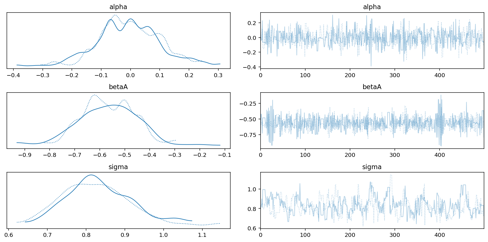
az.plot_trace(trace_5_X_M)
plt.tight_layout();

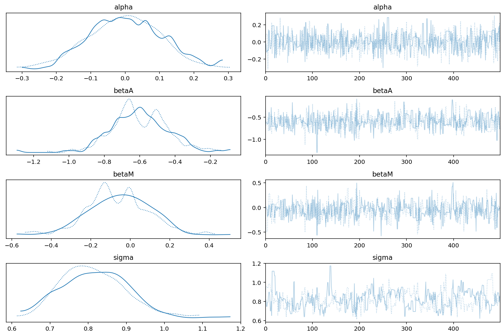
../_images/05_the_many_variables_and_the_spurious_waffles_65_0.png

az.plot_trace(trace_5_3_A)
plt.tight_layout()

../_images/05_the_many_variables_and_the_spurious_waffles_66_0.png

Code 5.20¶

A_seq = tf.linspace(-2.0, 2.0, num=30)
A_seq = tf.cast(A_seq, dtype=tf.float32)

Code 5.21¶

sample5X_alpha = posterior_5_X_M["alpha"][0]
sample5X_betaA = posterior_5_X_M["betaA"][0]
sample5X_sigma = posterior_5_X_M["sigma"][0]

# simulate M using A_seq
jdc_5_X_M_test = model_5_X_M(A_seq)

samples = jdc_5_X_M_test.sample(
    value=[sample5X_alpha, sample5X_betaA, sample5X_sigma, None]
)

M_sim = samples[-1]

M_sim.shape

TensorShape([500, 30])

# time to simulate D using M
sample53A_alpha = posterior_5_3_A["alpha"][0]
sample53A_betaA = posterior_5_3_A["betaA"][0]
sample53A_betaM = posterior_5_3_A["betaM"][0]
sample53A_sigma = posterior_5_3_A["sigma"][0]

jdc_5_3_A_test = model_5_3_A(A_seq, M_sim)

_, _, _, _, D_sim = jdc_5_3_A_test.sample(
    value=[sample53A_alpha, sample53A_betaA, sample53A_betaM, sample53A_sigma, None]
)

D_sim.shape

TensorShape([500, 30])

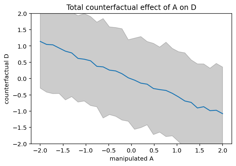
Code 5.22¶

# display counterfactual predictions
plt.plot(A_seq, tf.reduce_mean(D_sim, 0))
plt.gca().set(ylim=(-2, 2), xlabel="manipulated A", ylabel="counterfactual D")
plt.fill_between(
    A_seq, *tfp.stats.percentile(D_sim, q=(5.5, 94.5), axis=0), color="k", alpha=0.2
)
plt.title("Total counterfactual effect of A on D");

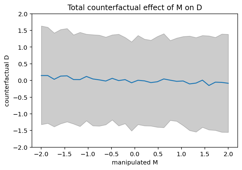
../_images/05_the_many_variables_and_the_spurious_waffles_73_0.png

Code 5.23¶

M_seq = tf.linspace(-2.0, 2.0, num=30)
M_seq = tf.cast(M_seq, dtype=tf.float32)


def compute_D_from_posterior_using_M(m):
    mu = sample53A_alpha + sample53A_betaM * m
    return tfd.Normal(loc=mu, scale=sample53A_sigma).sample()


D_sim = tf.transpose(
    tf.squeeze(tf.vectorized_map(compute_D_from_posterior_using_M, M_seq))
)
D_sim.shape

WARNING:tensorflow:Note that RandomStandardNormal inside pfor op may not give same output as inside a sequential loop.

TensorShape([500, 30])

# display counterfactual predictions
plt.plot(M_seq, tf.reduce_mean(D_sim, 0))
plt.gca().set(ylim=(-2, 2), xlabel="manipulated M", ylabel="counterfactual D")
plt.fill_between(
    M_seq, *tfp.stats.percentile(D_sim, q=(5.5, 94.5), axis=0), color="k", alpha=0.2
)
plt.title("Total counterfactual effect of M on D");

../_images/05_the_many_variables_and_the_spurious_waffles_76_0.png

Code 5.24, 5.25 and 5.26¶

Here the author explains how to do above manually in the overthinking box.

Due to the lack of Predictive support in tensorflow prob I had to do it anyways. So refer to above cells.

Code 5.27¶

Previous example used multiple predictors to show case spurious association but sometimes you do need multiple predictor variables as they do have influence on the outcome.

It is possible that one predictor variable is +ively related to outcome whereas the other one is -ively correlated.

We are going to use a new dataset called Milk.

Question that we want to answer is - To what extent energy content of milk, measured in KCal, is related to the percent of the brain mass that is neocortex.

d = RethinkingDataset.Milk.get_dataset()
d.info()
d.head()

<class 'pandas.core.frame.DataFrame'>
RangeIndex: 29 entries, 0 to 28
Data columns (total 8 columns):
 #   Column          Non-Null Count  Dtype  
---  ------          --------------  -----  
 0   clade           29 non-null     object 
 1   species         29 non-null     object 
 2   kcal.per.g      29 non-null     float64
 3   perc.fat        29 non-null     float64
 4   perc.protein    29 non-null     float64
 5   perc.lactose    29 non-null     float64
 6   mass            29 non-null     float64
 7   neocortex.perc  17 non-null     float64
dtypes: float64(6), object(2)
memory usage: 1.9+ KB

	clade	species	kcal.per.g	perc.fat	perc.protein	perc.lactose	mass	neocortex.perc
0	Strepsirrhine	Eulemur fulvus	0.49	16.60	15.42	67.98	1.95	55.16
1	Strepsirrhine	E macaco	0.51	19.27	16.91	63.82	2.09	NaN
2	Strepsirrhine	E mongoz	0.46	14.11	16.85	69.04	2.51	NaN
3	Strepsirrhine	E rubriventer	0.48	14.91	13.18	71.91	1.62	NaN
4	Strepsirrhine	Lemur catta	0.60	27.28	19.50	53.22	2.19	NaN

kcal.per.g - Kilocalories of energy per gram of milk
mass - Average female body mass, in KG
neocortex.perc - Percent of total brain mass that is neocortex mass

Although not mentioned in the question that was asked above, we are considering the female body mass as well. This is to see the masking that hides the relationships among the variables.

5.2 Masked relationship¶

Code 5.28¶

d["K"] = d["kcal.per.g"].pipe(lambda x: (x - x.mean()) / x.std())
d["N"] = d["neocortex.perc"].pipe(lambda x: (x - x.mean()) / x.std())
d["M"] = d.mass.pipe(np.log).pipe(lambda x: (x - x.mean()) / x.std())

tdf = dataframe_to_tensors("Milk", d, ["K", "N", "M"])

Code 5.29¶

A Simple Bivariate model between KCal and NeoCortex percent

# N => Standardized Neocortex percent


def model_5_5(neocortex_percent_std):
    def _generator():
        alpha = yield Root(
            tfd.Sample(tfd.Normal(loc=0.0, scale=1.0, name="alpha"), sample_shape=1)
        )
        betaN = yield Root(
            tfd.Sample(tfd.Normal(loc=0.0, scale=1.0, name="betaN"), sample_shape=1)
        )
        sigma = yield Root(
            tfd.Sample(tfd.Exponential(rate=1.0, name="sigma"), sample_shape=1)
        )

        mu = alpha + betaN * neocortex_percent_std

        K = yield tfd.Independent(
            tfd.Normal(loc=mu, scale=sigma, name="K"), reinterpreted_batch_ndims=1
        )

    return tfd.JointDistributionCoroutine(_generator, validate_args=True)


jdc_5_5 = model_5_5(tdf.N)

samples = jdc_5_5.sample()

samples

StructTuple(
  var0=<tf.Tensor: shape=(1,), dtype=float32, numpy=array([-0.4074485], dtype=float32)>,
  var1=<tf.Tensor: shape=(1,), dtype=float32, numpy=array([-0.38932118], dtype=float32)>,
  var2=<tf.Tensor: shape=(1,), dtype=float32, numpy=array([1.1790464], dtype=float32)>,
  var3=<tf.Tensor: shape=(29,), dtype=float32, numpy=
    array([ 0.59669876,         nan,         nan,         nan,         nan,
            1.6388006 ,  0.9897255 ,  1.2343845 ,         nan,  0.08673048,
            1.3017787 , -0.78627074, -1.7906513 ,         nan,         nan,
           -1.2799106 ,         nan,  0.2010594 ,         nan, -1.7962024 ,
                   nan, -0.9350649 ,         nan,  0.68466854, -1.9829096 ,
                   nan, -0.5187241 , -0.7603073 , -1.8256354 ], dtype=float32)>
)

If you see above displayed samples, you would see lot of NaN. Now tensorflow prob does not complain and/or throw an exception here but it is going to cause lot of pain.

In other words, we must not have this situation i.e. presence of NaN

Code 5.30¶

d["neocortex.perc"]

   55.16
     NaN
     NaN
     NaN
     NaN
   64.54
   64.54
   67.64
     NaN
   68.85
  58.85
  61.69
  60.32
    NaN
    NaN
  69.97
    NaN
  70.41
    NaN
  73.40
    NaN
  67.53
    NaN
  71.26
  72.60
    NaN
  70.24
  76.30
  75.49
Name: neocortex.perc, dtype: float64

We have lot of data missing in the neorcortex.perc colums

Code 5.31¶

Drop all the cases with missing values. This is known as COMPLETE CASE ANANLYSIS

dcc = d.iloc[d[["K", "N", "M"]].dropna(how="any", axis=0).index]

# we now have only 17 rows
dcc.describe()

	kcal.per.g	perc.fat	perc.protein	perc.lactose	mass	neocortex.perc	K	N	M
count	17.000000	17.000000	17.000000	17.000000	17.000000	17.000000	17.000000	1.700000e+01	17.000000
mean	0.657647	36.063529	16.255294	47.681176	16.637647	67.575882	0.098654	-2.821273e-15	0.033852
std	0.172899	14.705419	5.598480	13.585261	23.582322	5.968612	1.071235	1.000000e+00	1.138400
min	0.460000	3.930000	7.370000	27.090000	0.120000	55.160000	-1.125913	-2.080196e+00	-2.097830
25%	0.490000	27.180000	11.680000	37.800000	1.550000	64.540000	-0.940041	-5.086413e-01	-0.591039
50%	0.620000	37.780000	15.800000	46.880000	5.250000	68.850000	-0.134597	2.134697e-01	0.127441
75%	0.800000	50.490000	20.850000	55.200000	33.110000	71.260000	0.980633	6.172487e-01	1.212020
max	0.970000	55.510000	25.300000	70.770000	79.430000	76.300000	2.033906	1.461666e+00	1.727359

tdcc = dataframe_to_tensors("Milk", dcc, ["K", "N", "M"])

Code 5.32¶

jdc_5_5_draft = model_5_5(tdcc.N)

samples = jdc_5_5_draft.sample()

samples

StructTuple(
  var0=<tf.Tensor: shape=(1,), dtype=float32, numpy=array([1.7149136], dtype=float32)>,
  var1=<tf.Tensor: shape=(1,), dtype=float32, numpy=array([-1.3988794], dtype=float32)>,
  var2=<tf.Tensor: shape=(1,), dtype=float32, numpy=array([0.6669576], dtype=float32)>,
  var3=<tf.Tensor: shape=(17,), dtype=float32, numpy=
    array([ 4.85836   ,  2.4090662 ,  2.847961  ,  1.8739669 ,  1.9407496 ,
            3.4795122 ,  3.7360835 ,  3.4556942 ,  0.8344985 ,  1.0139198 ,
           -0.7194966 ,  1.5457227 ,  2.3558323 ,  0.13377067,  0.5906149 ,
           -0.72647536, -1.1218824 ], dtype=float32)>
)

You should not see an NaN in the samples

Code 5.33¶

Investigate if we have proper priors by plotting 50 prior regression lines

xseq = tf.constant([-2.0, 2.0], dtype=tf.float32)

sample_alpha, sample_betaN, sample_sigma, _ = model_5_5(xseq).sample(1000)

# we simply compute for the two possible values
mu_pred_0 = sample_alpha + sample_betaN * -2.0
mu_pred_1 = sample_alpha + sample_betaN * 2.0

mu_pred = tf.concat([mu_pred_0, mu_pred_1], axis=1)

plt.subplot(xlim=xseq.numpy(), ylim=xseq.numpy())
for i in range(50):
    plt.plot(xseq, mu_pred[i], "k", alpha=0.3)

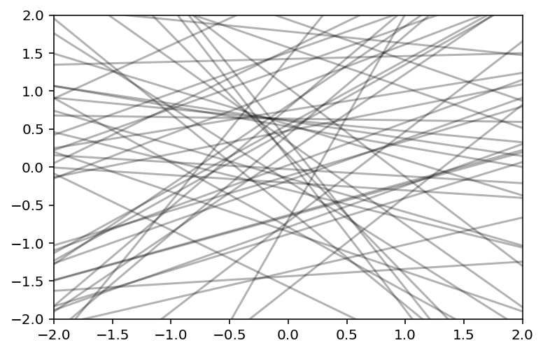
../_images/05_the_many_variables_and_the_spurious_waffles_97_0.png

Above does not look good. We should have better priors for \(\alpha\) so that it sticks closer to zero

Code 5.34¶

def model_5_5(neocortex_percent_std):
    def _generator():
        alpha = yield Root(
            tfd.Sample(tfd.Normal(loc=0.0, scale=0.2, name="alpha"), sample_shape=1)
        )
        betaN = yield Root(
            tfd.Sample(tfd.Normal(loc=0.0, scale=0.5, name="betaN"), sample_shape=1)
        )
        sigma = yield Root(
            tfd.Sample(tfd.Exponential(rate=1.0, name="sigma"), sample_shape=1)
        )

        mu = alpha + betaN * neocortex_percent_std

        K = yield tfd.Independent(
            tfd.Normal(loc=mu, scale=sigma, name="K"), reinterpreted_batch_ndims=1
        )

    return tfd.JointDistributionCoroutine(_generator, validate_args=True)


jdc_5_5 = model_5_5(tdcc.N)

posterior_5_5, trace_5_5 = sample_posterior(
    jdc_5_5, observed_data=(tdcc.K,), params=["alpha", "betaN", "sigma"]
)

Code 5.35¶

az.summary(trace_5_5, round_to=2, kind="stats", hdi_prob=0.89)

	mean	sd	hdi_5.5%	hdi_94.5%
alpha[0]	0.03	0.16	-0.23	0.29
betaN[0]	0.11	0.23	-0.25	0.48
sigma[0]	1.11	0.20	0.80	1.38

Code 5.36¶

xseq = tf.linspace(start=dcc.N.min() - 0.15, stop=dcc.N.max() + 0.15, num=30)
xseq = tf.cast(xseq, dtype=tf.float32)

sample_alpha = posterior_5_5["alpha"][0]
sample_betaN = posterior_5_5["betaN"][0]
sample_sigma = posterior_5_5["sigma"][0]

jdc_5_5_test = model_5_5(xseq)

ds, samples = jdc_5_5_test.sample_distributions(
    value=[sample_alpha, sample_betaN, sample_sigma, None]
)

mu_pred = ds[-1].distribution.loc

# summarize samples across cases
mu_mean = tf.reduce_mean(mu_pred, 0)
mu_PI = tfp.stats.percentile(mu_pred, q=(5.5, 94.5), axis=0)

az.plot_pair(dcc[["N", "K"]].to_dict(orient="list"))
plt.plot(xseq, mu_mean, "k")
plt.fill_between(xseq, mu_PI[0], mu_PI[1], color="k", alpha=0.2);

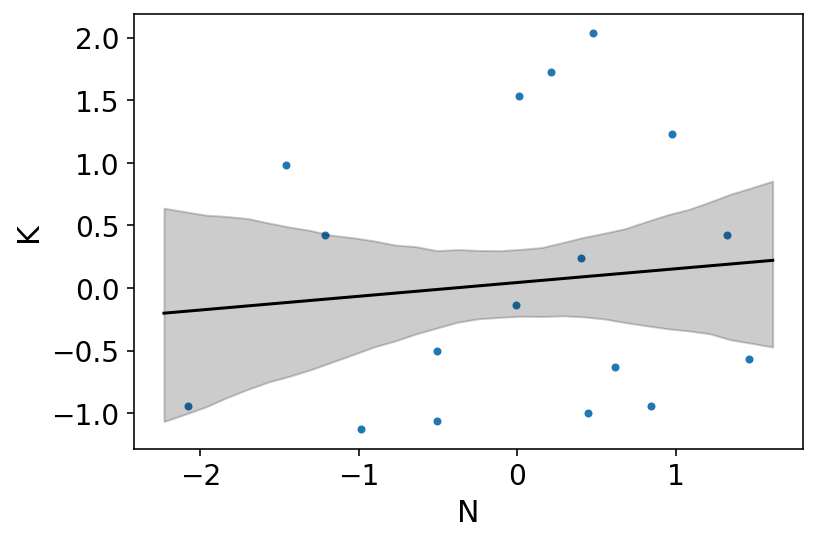
../_images/05_the_many_variables_and_the_spurious_waffles_104_0.png

Above plot displays weak association when using simple bivariate regression

Code 5.37¶

We now consider another predictor variable; the adult female body mass

def model_5_6(female_body_mass):
    def _generator():
        alpha = yield Root(
            tfd.Sample(tfd.Normal(loc=0.0, scale=0.2, name="alpha"), sample_shape=1)
        )
        betaM = yield Root(
            tfd.Sample(tfd.Normal(loc=0.0, scale=0.5, name="betaM"), sample_shape=1)
        )
        sigma = yield Root(
            tfd.Sample(tfd.Exponential(rate=1.0, name="sigma"), sample_shape=1)
        )

        mu = alpha + betaM * female_body_mass

        K = yield tfd.Independent(
            tfd.Normal(loc=mu, scale=sigma, name="K"), reinterpreted_batch_ndims=1
        )

    return tfd.JointDistributionCoroutine(_generator, validate_args=True)


jdc_5_6 = model_5_6(tdcc.M)

posterior_5_6, trace_5_6 = sample_posterior(
    jdc_5_6, observed_data=(tdcc.K,), params=["alpha", "betaM", "sigma"]
)

az.summary(trace_5_6, round_to=2, kind="stats", hdi_prob=0.89)

	mean	sd	hdi_5.5%	hdi_94.5%
alpha[0]	0.05	0.16	-0.19	0.31
betaM[0]	-0.26	0.26	-0.63	0.13
sigma[0]	1.07	0.21	0.75	1.39

Log-mass is negatively correlated with KCal. The influence is stronger than that of neocortex percent but it is in the opposite direction.

Code 5.38¶

Now let’s see what happens when we add both the predictor variables to the model

def model_5_7(neocortex_percent_std, female_body_mass):
    def _generator():
        alpha = yield Root(
            tfd.Sample(tfd.Normal(loc=0.0, scale=0.2, name="alpha"), sample_shape=1)
        )
        betaN = yield Root(
            tfd.Sample(tfd.Normal(loc=0.0, scale=0.5, name="betaN"), sample_shape=1)
        )
        betaM = yield Root(
            tfd.Sample(tfd.Normal(loc=0.0, scale=0.5, name="betaM"), sample_shape=1)
        )
        sigma = yield Root(
            tfd.Sample(tfd.Exponential(rate=1.0, name="sigma"), sample_shape=1)
        )

        mu = alpha + betaN * neocortex_percent_std + betaM * female_body_mass

        K = yield tfd.Independent(
            tfd.Normal(loc=mu, scale=sigma, name="K"), reinterpreted_batch_ndims=1
        )

    return tfd.JointDistributionCoroutine(_generator, validate_args=True)


jdc_5_7 = model_5_7(tdcc.N, tdcc.M)

posterior_5_7, trace_5_7 = sample_posterior(
    jdc_5_7, observed_data=(tdcc.K,), params=["alpha", "betaN", "betaM", "sigma"]
)

az.summary(trace_5_7, round_to=2, kind="stats", hdi_prob=0.89)

	mean	sd	hdi_5.5%	hdi_94.5%
alpha[0]	0.09	0.05	0.02	0.12
betaN[0]	0.05	0.35	-0.30	0.44
betaM[0]	-0.31	0.30	-0.70	-0.02
sigma[0]	0.61	0.56	0.04	1.19

By including both predictor variables in the regression, the posterior assocition of both with the outcome has increased.

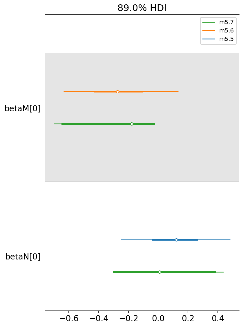
Code 5.39¶

coeftab = {"m5.5": trace_5_5, "m5.6": trace_5_6, "m5.7": trace_5_7}

az.plot_forest(
    list(coeftab.values()),
    model_names=list(coeftab.keys()),
    combined=True,
    var_names=["betaM", "betaN"],
    hdi_prob=0.89,
);

../_images/05_the_many_variables_and_the_spurious_waffles_113_0.png

Code 5.40¶

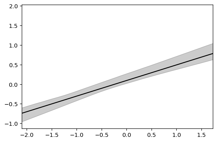
Counterfactual plot when setting N to zero and using M as the predictor variable

xseq = tf.linspace(start=dcc.M.min() - 0.15, stop=dcc.M.max() + 0.15, num=30)
xseq = tf.cast(xseq, dtype=tf.float32)

sample_alpha = posterior_5_7["alpha"][0]
sample_betaN = posterior_5_7["betaN"][0]
sample_betaM = posterior_5_7["betaN"][0]
sample_sigma = posterior_5_7["sigma"][0]

mu_pred = tf.transpose(
    tf.squeeze(tf.vectorized_map(lambda x: sample_alpha + sample_betaN * x, xseq))
)

# summarize samples across cases
mu_mean = tf.reduce_mean(mu_pred, 0)
mu_PI = tfp.stats.percentile(mu_pred, q=(5.5, 94.5), axis=0)

plt.subplot(xlim=(dcc.M.min(), dcc.M.max()), ylim=(dcc.K.min(), dcc.K.max()))
plt.plot(xseq, mu_mean, "k")
plt.fill_between(xseq, mu_PI[0], mu_PI[1], color="k", alpha=0.2);

../_images/05_the_many_variables_and_the_spurious_waffles_115_0.png

Code 5.41¶

# M -> K <- N
# M -> N
n = 100
M = tfd.Normal(loc=0.0, scale=1.0).sample((n,))
N = tfd.Normal(loc=M, scale=1.0).sample()
K = tfd.Normal(loc=N - M, scale=1.0).sample()

d_sim = pd.DataFrame({"K": K, "N": N, "M": M})

d_sim

	K	N	M
0	1.459018	-0.020620	0.279419
1	-1.647174	0.579855	1.110703
2	-1.408919	-1.536860	-0.877415
3	-1.942610	-1.388612	-0.556134
4	-1.078697	1.245790	0.408653
...	...	...	...
95	1.600822	2.254145	1.315559
96	-0.281205	-0.321023	0.331846
97	-1.464975	1.014630	1.981593
98	-1.260221	-1.304244	-0.143185
99	0.218382	-1.620139	-2.535684

100 rows × 3 columns

Code 5.42¶

# M -> K <- N
# N -> M
n = 100
N = tfd.Normal(loc=0.0, scale=1.0).sample((n,))
M = tfd.Normal(loc=N, scale=1.0).sample()
K = tfd.Normal(loc=N - M, scale=1.0).sample()

d_sim2 = pd.DataFrame({"K": K, "N": N, "M": M})

# M -> K <- N
# M <- U -> N
n = 100
N = tfd.Normal(loc=0.0, scale=1.0).sample((n,))
M = tfd.Normal(loc=M, scale=1.0).sample()
K = tfd.Normal(loc=N - M, scale=1.0).sample()

d_sim3 = pd.DataFrame({"K": K, "N": N, "M": M})

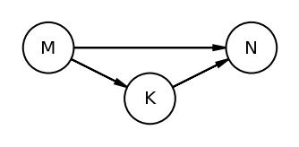
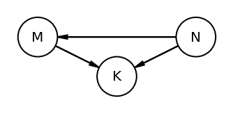
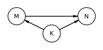
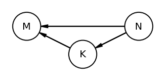
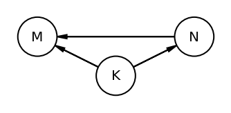
Code 5.43¶

The book uses dagitty an R package that can draw the DAG as well generate the equivalentDAGs given a DAG as input

At this point I do not have the corresponding function in python so I am manually specifying the equivalent DAGs (after seeing the result in RStudio as the book does not display the equivalentDAGs either)

coordinates = {"M": (0, 0.5), "K": (1, 1), "N": (2, 0.5)}
node_names = ["M", "K", "N"]

equivalent_dags = [
    [("M", "K"), ("N", "K"), ("M", "N")],
    [("M", "K"), ("K", "N"), ("M", "N")],
    [("M", "K"), ("N", "K"), ("N", "M")],
    [("K", "M"), ("K", "N"), ("M", "N")],
    [("K", "M"), ("N", "K"), ("N", "M")],
    [("K", "M"), ("K", "N"), ("N", "M")],
]

for e in equivalent_dags:
    dag = CausalGraphicalModel(nodes=node_names, edges=e)
    pgm = daft.PGM()
    for node in dag.dag.nodes:
        pgm.add_node(node, node, *coordinates[node])
    for edge in dag.dag.edges:
        pgm.add_edge(*edge)

    pgm.render()
    plt.gca().invert_yaxis()

../_images/05_the_many_variables_and_the_spurious_waffles_121_0.png

../_images/05_the_many_variables_and_the_spurious_waffles_121_1.png

../_images/05_the_many_variables_and_the_spurious_waffles_121_2.png

../_images/05_the_many_variables_and_the_spurious_waffles_121_3.png

../_images/05_the_many_variables_and_the_spurious_waffles_121_4.png

../_images/05_the_many_variables_and_the_spurious_waffles_121_5.png

Code 5.44¶

This section discusses Categorical Variables i.e. Discrete & Unordered variables.

We will again use HOWELL dataset here. In previous chapter, we had taken into consider sex variable and here we will model it as a categorical variable.

To start with let’s load the dataset

d = RethinkingDataset.Howell1.get_dataset()
d.info()
d.head()

<class 'pandas.core.frame.DataFrame'>
RangeIndex: 544 entries, 0 to 543
Data columns (total 4 columns):
 #   Column  Non-Null Count  Dtype  
---  ------  --------------  -----  
 0   height  544 non-null    float64
 1   weight  544 non-null    float64
 2   age     544 non-null    float64
 3   male    544 non-null    int64  
dtypes: float64(3), int64(1)
memory usage: 17.1 KB

	height	weight	age	male
0	151.765	47.825606	63.0	1
1	139.700	36.485807	63.0	0
2	136.525	31.864838	65.0	0
3	156.845	53.041914	41.0	1
4	145.415	41.276872	51.0	0

5.3 Categorical variables¶

Code 5.45¶

Here we are considering following model

\(h_i \sim Normal(\mu_i,\sigma)\)

\(\mu_i = \alpha + \beta_mm_i\)

\(\alpha \sim Normal(178,20)\)

\(\beta_m \sim Normal(0,10)\)

\(\sigma \sim Exponential(1)\)

m here is a categorical value and is 1 when we are dealing with males. This means that \(\alpha\) is used to predict both female and male heights.

But if we have a male then the height gets an extra \(\beta_m\). This also means that \(\alpha\) does not represent the average of all samples but rather the average of female height.

mu_female = tfd.Normal(loc=178.0, scale=20.0).sample((int(1e4),))

diff = tfd.Normal(loc=0.0, scale=10.0).sample((int(1e4),))

mu_male = tfd.Normal(loc=178.0, scale=20.0).sample((int(1e4),)) + diff

sample_dict = {"mu_female": mu_female.numpy(), "mu_male": mu_male.numpy()}

az.summary(az.from_dict(sample_dict), round_to=2, kind="stats", hdi_prob=0.89)

	mean	sd	hdi_5.5%	hdi_94.5%
mu_female	178.12	19.92	145.35	208.99
mu_male	178.00	22.56	142.61	214.34

The prior for male is wider (see std column). This is because it uses both the parameters.

Author explains that this makes assigning sensible priors harder. As show above, one of the category would have more uncertainity in the prediction as two priors are involved.

Code 5.46¶

Another approach is to use INDEX VARIABLE

d["sex"] = np.where(d.male.values == 1, 1, 0)
d.sex

    1
    0
    0
    1
    0
      ..
  1
  1
  0
  1
  1
Name: sex, Length: 544, dtype: int64

Code 5.47¶

tdf = dataframe_to_tensors("Howell1", d, {"height": tf.float32, "sex": tf.int32})


def model_5_8(sex):
    def _generator():
        alpha = yield Root(
            tfd.Sample(
                tfd.Normal(loc=178.0, scale=20.0, name="alpha"), sample_shape=(2,)
            )
        )
        sigma = yield Root(
            tfd.Sample(tfd.Uniform(low=0.0, high=50.0, name="sigma"), sample_shape=1)
        )

        # took long time to figure this out
        mu = tf.transpose(tf.gather(tf.transpose(alpha), sex))

        height = yield tfd.Independent(
            tfd.Normal(loc=mu, scale=sigma, name="height"), reinterpreted_batch_ndims=1
        )

    return tfd.JointDistributionCoroutine(_generator, validate_args=True)


jdc_5_8 = model_5_8(tdf.sex)

posterior_5_8, trace_5_8 = sample_posterior(
    jdc_5_8, observed_data=(tdf.height,), params=["alpha", "sigma"]
)

# now here is the special thing we have to do here
# alpha is actually a vector so for az_trace to display
# it properly I would have to extract it properly
female_alpha, male_alpha = tf.split(posterior_5_8["alpha"][0], 2, axis=1)

# reformatted
posterior_5_8_new = {
    "female_alpha": female_alpha.numpy(),
    "male_alpha": male_alpha.numpy(),
    "sigma": posterior_5_8["sigma"][0],
}

az.summary(az.from_dict(posterior_5_8_new), round_to=2, kind="stats", hdi_prob=0.89)

/opt/hostedtoolcache/Python/3.7.12/x64/lib/python3.7/site-packages/arviz/data/base.py:221: UserWarning: More chains (500) than draws (1). Passed array should have shape (chains, draws, *shape)
  UserWarning,

	mean	sd	hdi_5.5%	hdi_94.5%
female_alpha	134.92	1.10	133.44	136.71
male_alpha	142.59	0.72	141.52	143.83
sigma	27.41	0.81	26.16	28.71

Code 5.48¶

What is the expected difference between females and males ?

We can use the samples from the posterior to compute this.

posterior_5_8_new.update({"diff_fm": female_alpha.numpy() - male_alpha.numpy()})

az.summary(az.from_dict(posterior_5_8_new), round_to=2, kind="stats", hdi_prob=0.89)

/opt/hostedtoolcache/Python/3.7.12/x64/lib/python3.7/site-packages/arviz/data/base.py:221: UserWarning: More chains (500) than draws (1). Passed array should have shape (chains, draws, *shape)
  UserWarning,

	mean	sd	hdi_5.5%	hdi_94.5%
female_alpha	134.92	1.10	133.44	136.71
male_alpha	142.59	0.72	141.52	143.83
sigma	27.41	0.81	26.16	28.71
diff_fm	-7.67	1.28	-9.82	-5.77

Note that the above computation (i.e. diff) appeared in the arviz summary. This kind of calculation is called a CONTRAST.

Code 5.49¶

We explore the mile dataset again. We are now interested in clade variable which encodes the broad taxonomic membership of each species

d = RethinkingDataset.Milk.get_dataset()
d.clade.unique()

array(['Strepsirrhine', 'New World Monkey', 'Old World Monkey', 'Ape'],
      dtype=object)

Code 5.50¶

d["clade_id"] = d.clade.astype("category").cat.codes

d["clade_id"]

   3
   3
   3
   3
   3
   1
   1
   1
   1
   1
  1
  1
  1
  1
  2
  2
  2
  2
  2
  2
  0
  0
  0
  0
  0
  0
  0
  0
  0
Name: clade_id, dtype: int8

d.clade

      Strepsirrhine
      Strepsirrhine
      Strepsirrhine
      Strepsirrhine
      Strepsirrhine
   New World Monkey
   New World Monkey
   New World Monkey
   New World Monkey
   New World Monkey
  New World Monkey
  New World Monkey
  New World Monkey
  New World Monkey
  Old World Monkey
  Old World Monkey
  Old World Monkey
  Old World Monkey
  Old World Monkey
  Old World Monkey
               Ape
               Ape
               Ape
               Ape
               Ape
               Ape
               Ape
               Ape
               Ape
Name: clade, dtype: object

Based on above it seems that pandas is first sorting the categories by name and then assigning the number. So,

Ape = 0
New World Monkey = 1
Old World Monkey = 2
Strepsirrhine = 3

Code 5.51¶

We will now model again using the index variables

d["K"] = d["kcal.per.g"].pipe(lambda x: (x - x.mean()) / x.std())

tdf = dataframe_to_tensors("Milk", d, {"K": tf.float32, "clade_id": tf.int64})

CLADE_ID_LEN = len(set(d.clade_id.values))


def model_5_9(clade_id):
    def _generator():
        alpha = yield Root(
            tfd.Sample(
                tfd.Normal(loc=0.0, scale=0.5, name="alpha"),
                sample_shape=(CLADE_ID_LEN,),
            )
        )
        sigma = yield Root(
            tfd.Sample(tfd.Exponential(rate=1.0, name="sigma"), sample_shape=1)
        )

        mu = tf.transpose(
            tf.gather(tf.transpose(alpha), tf.cast(clade_id, dtype=tf.int64))
        )

        K = yield tfd.Independent(
            tfd.Normal(loc=mu, scale=sigma, name="K"), reinterpreted_batch_ndims=1
        )

    return tfd.JointDistributionCoroutine(_generator, validate_args=True)


jdc_5_9 = model_5_9(tdf.clade_id)

posterior_5_9, trace_5_9 = sample_posterior(
    jdc_5_9, observed_data=(tdf.K,), params=["alpha", "sigma"]
)

# now here is the special thing we have to do here
# alpha is actually a vector so for az_trace to display
# it properly I would have to extract it properly
ape_alpha, nwm_alpha, owm_alpha, strep_alpha = tf.split(
    posterior_5_9["alpha"][0], 4, axis=1
)

# reformatted
updated_posterior_5_9 = {
    "ape_alpha": ape_alpha.numpy(),
    "nwm_alpha": nwm_alpha.numpy(),
    "owm_alpha": owm_alpha.numpy(),
    "strep_alpha": strep_alpha.numpy(),
    "sigma": posterior_5_9["sigma"][0],
}

az.summary(az.from_dict(updated_posterior_5_9), round_to=2, kind="stats", hdi_prob=0.89)

/opt/hostedtoolcache/Python/3.7.12/x64/lib/python3.7/site-packages/arviz/data/base.py:221: UserWarning: More chains (500) than draws (1). Passed array should have shape (chains, draws, *shape)
  UserWarning,

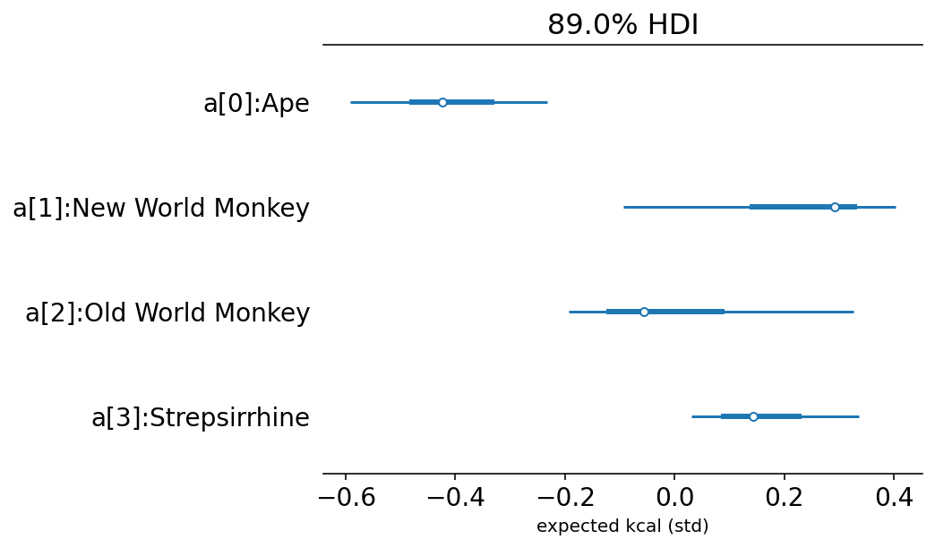
	mean	sd	hdi_5.5%	hdi_94.5%
ape_alpha	-0.42	0.11	-0.59	-0.23
nwm_alpha	0.22	0.16	-0.09	0.40
owm_alpha	-0.01	0.16	-0.19	0.33
strep_alpha	0.16	0.10	0.03	0.34
sigma	1.03	0.13	0.83	1.23

labels = ["a[" + str(i) + "]:" + s for i, s in enumerate(sorted(d.clade.unique()))]
az.plot_forest({"a": trace_5_9.posterior["alpha"].values[0][None, ...]}, hdi_prob=0.89)
plt.gca().set(yticklabels=labels[::-1], xlabel="expected kcal (std)");

../_images/05_the_many_variables_and_the_spurious_waffles_143_0.png

Code 5.52¶

np.random.seed(63)
d["house"] = np.random.choice(np.repeat(np.arange(4), 8), d.shape[0], False)

d.house

   2
   3
   1
   3
   0
   0
   0
   2
   0
   0
  1
  3
  1
  1
  3
  1
  2
  0
  3
  2
  3
  0
  3
  1
  3
  2
  0
  2
  2
Name: house, dtype: int64

Code 5.53¶

tdf = dataframe_to_tensors(
    "Milk", d, {"K": tf.float32, "clade_id": tf.int32, "house": tf.int32}
)

CLADE_ID_LEN = len(set(d.clade_id.values))
HOUSE_ID_LEN = len(set(d.house.values))


def model_5_10(clade_id, house_id):
    def _generator():
        alpha = yield Root(
            tfd.Sample(
                tfd.Normal(loc=0.0, scale=0.5, name="alpha"),
                sample_shape=(CLADE_ID_LEN,),
            )
        )
        house = yield Root(
            tfd.Sample(
                tfd.Normal(loc=0.0, scale=0.5, name="house"),
                sample_shape=(HOUSE_ID_LEN,),
            )
        )
        sigma = yield Root(
            tfd.Sample(tfd.Exponential(rate=1.0, name="sigma"), sample_shape=1)
        )

        mu = tf.transpose(
            tf.gather(tf.transpose(alpha), tf.cast(clade_id, dtype=tf.int64))
        ) + tf.transpose(tf.gather(tf.transpose(house), house_id))

        K = yield tfd.Independent(
            tfd.Normal(loc=mu, scale=sigma, name="K"), reinterpreted_batch_ndims=1
        )

    return tfd.JointDistributionCoroutine(_generator, validate_args=True)


jdc_5_10 = model_5_10(tdf.clade_id, tdf.house)

posterior_5_10, trace_5_10 = sample_posterior(
    jdc_5_10, observed_data=(tdf.K,), params=["alpha", "house", "sigma"]
)

# now here is the special thing we have to do here
# alpha is actually a vector so for az_trace to display
# it properly I would have to extract it properly
ape_alpha, nwm_alpha, owm_alpha, strep_alpha = tf.split(
    posterior_5_10["alpha"][0], 4, axis=1
)
house_0, house_1, house_2, house_3 = tf.split(posterior_5_10["house"][0], 4, axis=1)

# reformatted
updated_posterior_5_10 = {
    "ape_alpha": ape_alpha.numpy(),
    "nwm_alpha": nwm_alpha.numpy(),
    "owm_alpha": owm_alpha.numpy(),
    "strep_alpha": strep_alpha.numpy(),
    "house_0": house_0.numpy(),
    "house_1": house_1.numpy(),
    "house_2": house_2.numpy(),
    "house_3": house_3.numpy(),
    "sigma": posterior_5_10["sigma"][0],
}

az.summary(
    az.from_dict(updated_posterior_5_10), round_to=2, kind="stats", hdi_prob=0.89
)

/opt/hostedtoolcache/Python/3.7.12/x64/lib/python3.7/site-packages/arviz/data/base.py:221: UserWarning: More chains (500) than draws (1). Passed array should have shape (chains, draws, *shape)
  UserWarning,

	mean	sd	hdi_5.5%	hdi_94.5%
ape_alpha	-0.50	0.28	-0.91	-0.06
nwm_alpha	0.30	0.29	-0.10	0.77
owm_alpha	0.62	0.30	0.20	1.10
strep_alpha	-0.53	0.33	-1.03	0.01
house_0	0.20	0.28	-0.29	0.59
house_1	0.00	0.35	-0.54	0.43
house_2	0.20	0.31	-0.31	0.66
house_3	-0.29	0.29	-0.73	0.09
sigma	0.77	0.11	0.58	0.91

Statistical Rethinking (2nd Edition)

5. The Many Variables & The Spurious Waffles

Contents

5. The Many Variables & The Spurious Waffles¶

5.1 Spurious association¶

Code 5.1¶

Code 5.2¶

Code 5.3¶

Code 5.4¶

Code 5.5¶

Code 5.6¶

Code 5.7¶

Code 5.8¶

Code 5.9¶

Code 5.10¶

Code 5.11¶

Code 5.12 (TODO)¶

Code 5.13¶

Code 5.14¶

Code 5.15¶

Code 5.16¶

Code 5.17¶

Code 5.18¶

Code 5.19¶

Code 5.20¶

Code 5.21¶

Code 5.22¶

Code 5.23¶

Code 5.24, 5.25 and 5.26¶

Code 5.27¶

5.2 Masked relationship¶

Code 5.28¶

Code 5.29¶

Code 5.30¶

Code 5.31¶

Code 5.32¶

Code 5.33¶

Code 5.34¶

Code 5.35¶

Code 5.36¶

Code 5.37¶

Code 5.38¶

Code 5.39¶

Code 5.40¶

Code 5.41¶

Code 5.42¶

Code 5.43¶

Code 5.44¶

5.3 Categorical variables¶

Code 5.45¶

Code 5.46¶

Code 5.47¶

Code 5.48¶

Code 5.49¶

Code 5.50¶

Code 5.51¶

Code 5.52¶

Code 5.53¶