![]()
1.1 Example: Polynomial Curve Fitting
import os
import functools
import numpy as np

import pandas as pd
import matplotlib.pyplot as plt

from sklearn.preprocessing import PolynomialFeatures

if "OUTPUT_RETINA_IMAGES" in os.environ:
    %config InlineBackend.figure_format = "retina"

plt.rcParams["axes.spines.right"] = False
plt.rcParams["axes.spines.top"] = False
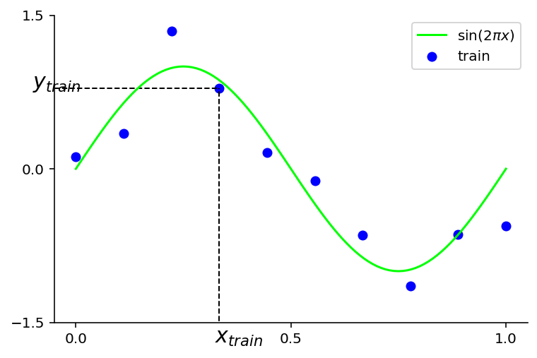
We generate a dataset using \(sin(2\pi x)\) function but also add some observation noise to reflect the true world !
N = 10
SEED = 1234
SCALE = 0.25

np.random.seed(SEED)

def true_fun(x):
    return np.sin(2 * np.pi * x)

def generate_noisy_data(x, scale=SCALE):
    y = true_fun(x) + np.random.normal(scale=scale, size=x.shape)
    return y

x_plot = np.arange(0, 1.01, 0.01)
y_plot = true_fun(x_plot)

# points with noise, will act as train data
x_train = np.linspace(0, 1, N)
y_train = generate_noisy_data(x_train)

plt.plot(x_plot, y_plot, color='lime', label="$\sin(2\pi x)$")
plt.scatter(x_train, y_train, marker='o', color='blue', label="train")
plt.hlines(y=y_train[3], xmin=-2, xmax=x_train[3], linewidth=1, linestyle='--', color = 'k')
plt.vlines(x=x_train[3], ymin=-2, ymax=y_train[3], linewidth=1, linestyle='--', color = 'k')

plt.text(-0.1, y_train[3], "$y_{train}$", fontsize=15)
plt.text(x_train[3] - 0.01, -1.7, "$x_{train}$", fontsize=15)
plt.yticks( [-1.5, 0.0, 1.5] )
plt.xticks( [0.0, 0.5, 1.0] )
plt.xlim(-0.05, 1.05)
plt.ylim(-1.5, 1.5)
plt.legend();
We will now use different models of regression to determine the weights. These models will differ by the degree of polynomial so as a first step let’s transform our features (\(x_{train}\))
def transform_features(X, m):
    """ Create a polynomial of specified degrees """
    return PolynomialFeatures(degree=m).fit_transform(X.reshape(-1, 1))

# examples of creating the polynomial features
features_m_0 = transform_features(x_train, m=0)
features_m_1 = transform_features(x_train, m=1)
features_m_3 = transform_features(x_train, m=3)
features_m_9 = transform_features(x_train, m=9)
def multiple_regression_fit(features, y_train):
    A_t = features.T @ features
    weight_vector = np.linalg.solve(A_t, features.T @ y_train)
    return weight_vector

def multiple_regression_predict(features, weight_vector):
    return np.dot(features, weight_vector)
# we will invoke above fit & predict methods in a loop for all
# the polynomials

# test data
# x that we used to draw out sin function will act as the test data

def regress(m, x, y):
    poly_train_features = transform_features(x, m=m)
    return multiple_regression_fit(poly_train_features, y)

def predict(m, x, weight_vector):
    poly_test_features = transform_features(x, m=m)
    return multiple_regression_predict(poly_test_features, weight_vector)

def regress_and_predict(m, x_train, y_train, x_test):
    weight_vector = regress(m, x_train, y_train)
    return predict(m, x_test, weight_vector)

fig, ax = plt.subplots(2, 2, sharex=True, sharey=True)

plt.xlim(-0.05, 1.05)
plt.ylim(-1.5, 1.5)

def plot(m, x, y_predict, ax):
    # true function
    ax.plot(x_plot, y_plot, color='lime', label="$\sin(2\pi x)$")

    # training data
    ax.scatter(x_train, y_train, marker='o', color='blue', label="Train")

    # Show the poly degree
    ax.text(0.65, 0.8, f"M={m}")

    # finally the predictions
    ax.plot(x, y_predict, color='red', label="Test")


x_test = np.linspace(0, 1, 100)
y_test = generate_noisy_data(x_test)

partial_rp = functools.partial(regress_and_predict,
                        x_train=x_train,
                        y_train=y_train,
                        x_test=x_test)

results = list(map(partial_rp, [0,1,3,9]))

plot(m=0, x=x_test, y_predict=results[0], ax=ax[0][0])
plot(m=1, x=x_test, y_predict=results[1], ax=ax[0][1])
plot(m=3, x=x_test, y_predict=results[2], ax=ax[1][0])
plot(m=9, x=x_test, y_predict=results[3], ax=ax[1][1])

plt.legend(bbox_to_anchor=(1.05, 1.05));
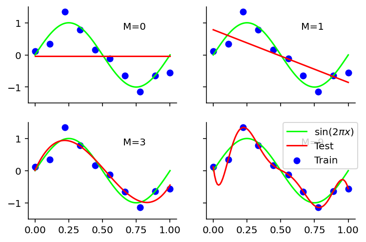
Notes -
Red curve shows the fitted curve.
M=0 fails to create the sin curve
M=1 also failed
M=3 seems to re-create the curve close to original function
M=9 creates a curve that passes through all the training data but fails to approximate sin and is very wiggly. This is overfitting.
Evaluating residual value of \(E(w^*)\)
def rmse(a, b):
    return np.sqrt(np.mean(np.square(a - b)))

# try polynomial of degrees from 0 to 10
M = range(0, 10)

weight_vectors = []
for m in M:
    w = regress(m=m, x=x_train, y=y_train)
    weight_vectors.append(w)

def compute_errors(x, y, m, weight_vector):
    y_predict = predict(m=m, x=x, weight_vector=weight_vector)
    return rmse(y_predict, y)

def accumate_errors(x, y):
    m_w = zip(M, weight_vectors)
    errors = []
    for (m, w) in m_w:
        errors.append(compute_errors(x, y, m, w))
    return errors

x_test = np.arange(0, 1.01, 0.01)
y_test = generate_noisy_data(x_test)

training_errors = accumate_errors(x_train, y_train)
test_errors = accumate_errors(x_test, y_test)

plt.plot(training_errors, 'o-', mfc="none", mec="b", ms=10, c="b", label="Training")
plt.plot(test_errors, 'o-', mfc="none", mec="r", ms=10, c="r", label="Test")
plt.legend()
plt.yticks( [0,0.5,1] )
plt.xticks( [0,3,6,9] )
plt.xlabel("degree")
plt.ylabel("RMSE");
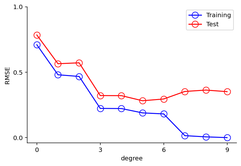
Notes -
For M = 9, the training set error goes to zero, for test set it shoots up
A polynomial of higher degree contains the functions for lower so why this behavior ?
Inspecting the weight vectors of various polynomials
weight_vector_m_0 = regress(m=0, x=x_train, y=y_train)
weight_vector_m_1 = regress(m=1, x=x_train, y=y_train)
weight_vector_m_3 = regress(m=3, x=x_train, y=y_train)
weight_vector_m_9 = regress(m=9, x=x_train, y=y_train)

# makeing them same dimension so
# as display using a pandas frame
def pad_weight_vectors(weight_vector):
    while len(weight_vector) <= 9:
        weight_vector = np.append(weight_vector, 0.)
    return weight_vector

weight_vector_m_0 = pad_weight_vectors(weight_vector_m_0)
weight_vector_m_1 = pad_weight_vectors(weight_vector_m_1)
weight_vector_m_3 = pad_weight_vectors(weight_vector_m_3)
weight_vector_m_9 = pad_weight_vectors(weight_vector_m_9)

df = pd.DataFrame([weight_vector_m_0,weight_vector_m_1,weight_vector_m_3,weight_vector_m_9]).transpose()
df.columns = ['M=0', 'M=1', 'M=3', 'M=9']

df
| M=0 | M=1 | M=3 | M=9 | |
|---|---|---|---|---|
| 0 | -0.035921 | 0.783019 | 0.011334 | 0.117859 |
| 1 | 0.000000 | -1.637881 | 9.292162 | -32.239388 |
| 2 | 0.000000 | 0.000000 | -26.789442 | 552.759807 |
| 3 | 0.000000 | 0.000000 | 17.037287 | -2730.224980 |
| 4 | 0.000000 | 0.000000 | 0.000000 | 4770.532869 |
| 5 | 0.000000 | 0.000000 | 0.000000 | 2010.207069 |
| 6 | 0.000000 | 0.000000 | 0.000000 | -19325.059542 |
| 7 | 0.000000 | 0.000000 | 0.000000 | 28349.068583 |
| 8 | 0.000000 | 0.000000 | 0.000000 | -17838.530474 |
| 9 | 0.000000 | 0.000000 | 0.000000 | 4242.807525 |
Notes -
As M increases, the magnitude of weights is becoming larger
In particular for M=9, the weights become very large +ive and -ive so that corresponding polynomial function matches the data point exactly
Intuitively, what is happening is that the more flexible polynomials with larger values of M are becoming increasingly tuned to the random noise on the target values
Increasing the datasize reduces overfitting
Here we use M=9 that resulted in overfitting but increase the training dataset size. We will try N=15 and N=100.
def analyze_overfit(N, m=9):
    x_train = np.linspace(0, 1, N)
    y_train = generate_noisy_data(x_train)

    poly_train_features = transform_features(x_train, m=m)
    weight_vector = multiple_regression_fit(poly_train_features, y_train)

    return x_train, y_train, weight_vector

def regress_and_plot(x):

    fig, ax = plt.subplots(1, 2, sharey=True, figsize=(10, 4))

    plt.xlim(-0.05, 1.05)
    plt.ylim(-2.0, 2.0)

    for i, n in enumerate([15, 100]):
        # get weight vector
        x_train, y_train, weight_vector = analyze_overfit(N=n)
        # make predictions
        poly_test_features = transform_features(x, m=9)
        y_predict = multiple_regression_predict(poly_test_features, weight_vector)

        # true function
        ax[i].plot(x_plot, y_plot, color='lime', label="$\sin(2\pi x)$")

        # training data
        ax[i].scatter(x_train, y_train, marker='o', color='blue', label="Train")

        # Show the poly degree
        ax[i].text(0.65, 0.8, f"N={n}")

        # finally the predictions
        ax[i].plot(x, y_predict, color='red', label="Test")

regress_and_plot(x=x_test)
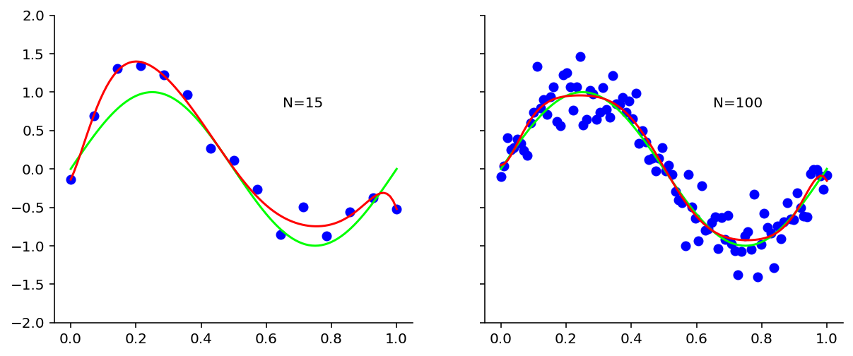
From the above plots, it is evident that as we increased the data size to 100, we got rid of overfitting.
One rough heuristic that is sometimes advocated is that the number of data points should be no less than some multiple (say 5 or 10) of the number of adaptive parameters in the model.
It is indeed a nuisance to have this delicate dance between number of parameters and dataset size. Could Bayesian Inference help ? Authors says - Yes
At the moment we restrict ourselves to current situation only. Here because we had a synthetic dataset we could increase the number of training samples at will but real world is differnt. So next question to ask is - Could we reduce overfitting when we have less number of training examples ?
Regularization
We observed that the weights started to reach larger values for M=9; so one technique to circumvent is to add penalty term to the error function in order to discouragethe coefficients from reaching large values.
The new error function then takes the form
The \(\lambda\) in the above equation controls the contribution of the regularization to the overall error. This is a hyper-parameter.
Above can be done in closed form.
This method is known by various other names as well.
In statistics, it is known as shrinkage since we are reducing the values of \(\mathbf{w}\).
In machine learning, we call it weight decay.
In this particular case of quadratics weight decay, it is also called Ridge Regression
After some mathematical rigor, the closed form solution is -
# we will modify our multiple regression fit function
# to take this into account. Rest of the functions defined above
# should still be usable

def multiple_regression_ridge_fit(features, y_train, lamb):
    # Note - addition of second term for A_t
    A_t = features.T @ features + lamb * np.eye(features.shape[1], features.shape[1])
    weight_vector = np.linalg.solve(A_t, features.T @ y_train)
    return weight_vector

def regress_ridge(m, x, y, lamb):
    poly_train_features = transform_features(x, m=m)
    # get weights
    weight_vector = multiple_regression_ridge_fit(poly_train_features, y, lamb)
    return weight_vector

def regress_ridge_and_plot(x):

    fig, ax = plt.subplots(1, 3, sharey=True, figsize=(10,4))

    plt.xlim(-0.05, 1.05)
    plt.ylim(-2.0, 2.0)

    for i, lamb in enumerate([-1000, -18, 0]):

        weight_vector_m_9_ridge = regress_ridge(m=9, x=x_train, y=y_train, lamb=np.exp(lamb))
        y_predict = predict(m=9, x=x, weight_vector=weight_vector_m_9_ridge)

        # true function
        ax[i].plot(x_plot, y_plot, color='lime', label="$\sin(2\pi x)$")

        # training data
        ax[i].scatter(x_train, y_train, marker='o', color='blue', label="Train")

        # Show the poly degree
        ax[i].text(0.65, 0.8, f"$ln \ \lambda$={lamb}")

        # finally the predictions
        ax[i].plot(x, y_predict, color='red', label="Test")

regress_ridge_and_plot(x=x_test)
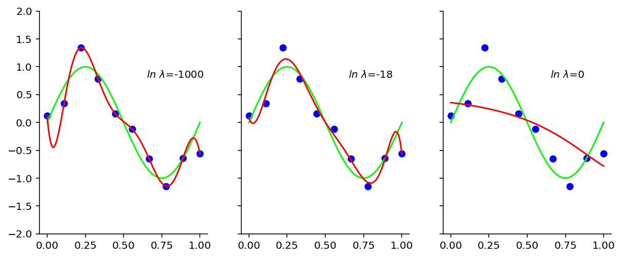
\(ln \ \lambda\) = -1000 corresponds to having no regualrizer. In the above plot, are shown the effect of 3 different regularizers. Clearly out of these 3, \(ln \ \lambda\) = -18 seems to do the trick
weight_vector_m_9_0 = regress_ridge(m=9, x=x_train, y=y_train, lamb=np.exp(-1000))
weight_vector_m_9_1 = regress_ridge(m=9, x=x_train, y=y_train, lamb=np.exp(-18))
weight_vector_m_9_2 = regress_ridge(m=9, x=x_train, y=y_train, lamb=np.exp(0))

weight_vector_m_9_0 = pad_weight_vectors(weight_vector_m_9_0)
weight_vector_m_9_1 = pad_weight_vectors(weight_vector_m_9_1)
weight_vector_m_9_2 = pad_weight_vectors(weight_vector_m_9_2)

df = pd.DataFrame([weight_vector_m_9_0,weight_vector_m_9_1,weight_vector_m_9_2]).transpose()
df.columns = ['ln lambda=-1000', 'ln lambda=-18', 'ln lambda=0', ]

df
| ln lambda=-1000 | ln lambda=-18 | ln lambda=0 | |
|---|---|---|---|
| 0 | 0.117859 | 0.084455 | 0.357091 |
| 1 | -32.239388 | -8.198305 | -0.332004 |
| 2 | 552.759807 | 185.185113 | -0.403486 |
| 3 | -2730.224980 | -860.896425 | -0.304300 |
| 4 | 4770.532869 | 1438.245455 | -0.191590 |
| 5 | 2010.207069 | -422.121845 | -0.097300 |
| 6 | -19325.059542 | -1042.178585 | -0.023986 |
| 7 | 28349.068583 | 231.682032 | 0.031876 |
| 8 | -17838.530474 | 1113.582844 | 0.074296 |
| 9 | 4242.807525 | -635.940163 | 0.106591 |
We see that, as the value of \(\lambda\) increases, the typical magnitude of the coefficients gets smaller
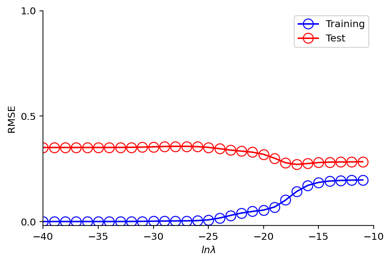
lamb = range(-40, -10, 1)

train_errors = []
test_errors = []
for l in lamb:
    weight_vector_m_9_ridge = regress_ridge(m=9, x=x_train, y=y_train, lamb=np.exp(l))

    y_train_predict = predict(m=9, x=x_train, weight_vector=weight_vector_m_9_ridge)
    y_test_predict = predict(m=9, x=x_test, weight_vector=weight_vector_m_9_ridge)

    train_errors.append(rmse(y_train, y_train_predict))
    test_errors.append(rmse(y_test, y_test_predict))

plt.plot(lamb, train_errors, 'o-', mfc="none", mec="b", ms=10, c="b", label="Training")
plt.plot(lamb, test_errors, 'o-', mfc="none", mec="r", ms=10, c="r", label="Test")
plt.legend()
plt.yticks( [0,0.5,1] )
plt.xlim((-40, -10))
plt.xlabel("$ln \lambda$")
plt.ylabel("RMSE");